An employment analyst studies the trends in employment in three industries across five years (60 months). The analyst performs ARIMA to fit a model for the trade industry.
- Open the sample data, EmploymentTrends.MWX.
- Choose .
- In Series, enter Trade.
- In Autoregressive, under Nonseasonal, enter 1.
- Click Graphs, then select ACF of residuals.
- Click OK.
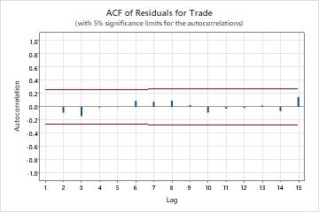
Interpret the results
The autoregressive term has a p-value that is less than the significance level of 0.05. The
analyst concludes that the coefficient for the autoregressive term is statistically
different from 0, and keeps the term in the model. The p-values for the Ljung-Box
chi-square statistics are all greater than 0.05, and none of the correlations for
the autocorrelation function of the residuals are significant. The analyst concludes
that the model meets the assumption that the residuals are independent.
Estimates at Each Iteration
| Iteration | SSE | Parameters | |
|---|---|---|---|
| 0 | 543.908 | 0.100 | 90.090 |
| 1 | 467.180 | -0.050 | 105.068 |
| 2 | 412.206 | -0.200 | 120.046 |
| 3 | 378.980 | -0.350 | 135.024 |
| 4 | 367.545 | -0.494 | 149.372 |
| 5 | 367.492 | -0.503 | 150.341 |
| 6 | 367.492 | -0.504 | 150.410 |
| 7 | 367.492 | -0.504 | 150.415 |
Final Estimates of Parameters
| Type | Coef | SE Coef | T-Value | P-Value |
|---|---|---|---|---|
| AR 1 | -0.504 | 0.114 | -4.42 | 0.000 |
| Constant | 150.415 | 0.325 | 463.34 | 0.000 |
| Mean | 100.000 | 0.216 |
Number of observations: 60
Residual Sums of Squares
| DF | SS | MS |
|---|---|---|
| 58 | 366.733 | 6.32299 |
Modified Box-Pierce (Ljung-Box) Chi-Square Statistic
| Lag | 12 | 24 | 36 | 48 |
|---|---|---|---|---|
| Chi-Square | 4.05 | 12.13 | 25.62 | 32.09 |
| DF | 10 | 22 | 34 | 46 |
| P-Value | 0.945 | 0.955 | 0.849 | 0.940 |