A reliability engineer wants to investigate electrical current leakage between transistors in an electronic device. When current leakage reaches a certain threshold value, the electronic device fails. To accelerate failures for testing, the devices were tested under much higher than normal temperatures. Devices were inspected for failure every two days.
The engineer performs an accelerated life test to estimate the time until failure for the device under normal operating conditions (55° C) and worst-case operating conditions (85° C). The engineer wants to determine the B5 life, which is the estimated amount of time until 5% of the devices are expected to fail.
- Open the sample data, CurrentLeakage.MWX.
- Choose .
- Select Responses are uncens/arbitrarily censored data.
- In Variables/Start variables, enter StartTime.
- In End variables, enter EndTime.
- In Freq. columns, enter Count.
- In Accelerating var, enter Temp.
- From Relationship, select Arrhenius.
- From Assumed distribution, select Weibull.
- Click Estimate. Under Percentile and Probability Estimation, select Enter new predictor values, then enter NewTemp.
- In Estimate percentiles for percents, enter 5, then click OK.
- Click Graphs. In Design value to include on plots, enter 55.
- Under Relation plot, in Plot percentiles for percents, enter 5, then select Display failure times on plot.
- Click OK in each dialog box.
Interpret the results
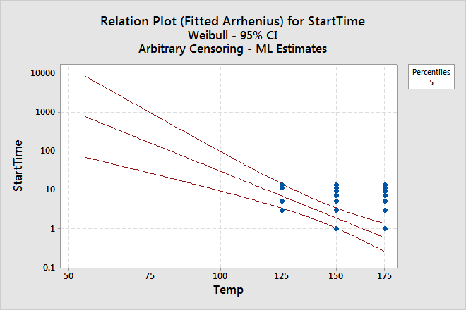
Based on the results in the table of percentiles, the engineer can conclude the following:
- At the design temperature (55° C), 5% of the devices will fail after approximately 760 days (slightly over 2 years).
- At the worst-case temperature (85° C), 5% of the devices will fail after approximately 81 days.
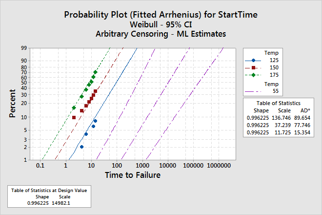
The probability plot based on the fitted model can help you determine whether the distribution, transformation, and assumption of equal shape (Weibull) at each level of the accelerating variable are appropriate. For these data, the points follow an approximate straight line. Therefore, assumptions of the model are appropriate for the accelerating variable levels.
Censoring
| Censoring Information | Count |
|---|---|
| Right censored value | 95 |
| Interval censored value | 58 |
Regression Table
| Standard Error | 95.0% Normal CI | |||||
|---|---|---|---|---|---|---|
| Predictor | Coef | Z | P | Lower | Upper | |
| Intercept | -17.0990 | 4.13633 | -4.13 | 0.000 | -25.2061 | -8.99195 |
| Temp | 0.755405 | 0.157076 | 4.81 | 0.000 | 0.447542 | 1.06327 |
| Shape | 0.996225 | 0.136187 | 0.762071 | 1.30232 | ||
Table of Percentiles
| Standard Error | 95.0% Normal CI | ||||
|---|---|---|---|---|---|
| Percent | Temp | Percentile | Lower | Upper | |
| 5 | 55 | 759.882 | 928.717 | 69.2500 | 8338.21 |
| 5 | 85 | 81.0926 | 63.2317 | 17.5897 | 373.855 |