A medical researcher wants to know how the dosage level of a new medicine affects the presence of bacteria in adults. The researcher conducts an experiment with 30 patients and 6 dosage levels. For two weeks, the researcher gives one dosage level to 5 patients, another dosage level to another 5 patients, and so on. At the end of the two-week period, each patient is tested to determine whether any bacteria are detected.
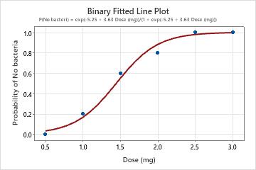
Because the data include a binary response and one continuous predictor, the researcher uses a binary fitted line plot to determine whether the dosage of a medicine is related to the presence of bacteria.
Choose Stat > Regression > Binary Fitted Line Plot.
From the drop-down list, select Response in event/trial format.
In Event name, type No bacteria.
In Number of events, enter 'No Bacteria'.
In Number of trials, enter Trials.
In Predictor, enter 'Dose (mg)'.
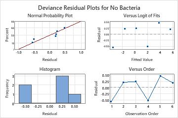
Click Graphs. Under Residual Plots, select Four in one.
Click OK in each dialog box.
Interpret the results
The p-value for the medicine dosage is less than the significance level of 0.05. These results indicate that the relationship between the dosage of medicine and the presence of bacteria is statistically significant. The binary fitted line plot shows that as the amount of dosage increases, the likelihood that no bacteria is present increases. Furthermore, the odds ratio indicates that for every 1 mg increase in the dosage level, the likelihood that no bacteria is present increases by approximately 38 times. The fitted line plot shows the model fits the data well and the residual plots do not show any problems with the model.