In This Topic
Step 1: Determine whether the differences between group means are statistically significant
- P-value ≤ α: The differences between some of the means are statistically significant
- If the p-value is less than or equal to the significance level, you reject the null hypothesis and conclude that not all population means are equal. Use your specialized knowledge to determine whether the differences are practically significant. For more information, go to Statistical and practical significance.
- P-value > α: The differences between the means are not statistically significant
- If the p-value is greater than the significance level, you do not have enough evidence to reject the null hypothesis that the population means are all equal. Verify that your test has enough power to detect a difference that is practically significant. For more information, go to Increase the power of a hypothesis test.
Analysis of Variance
| Source | DF | Adj SS | Adj MS | F-Value | P-Value |
|---|---|---|---|---|---|
| Paint | 3 | 281.7 | 93.90 | 6.02 | 0.004 |
| Error | 20 | 312.1 | 15.60 | ||
| Total | 23 | 593.8 |
Key Result: P-Value
In these results, the null hypothesis states that the mean hardness values of 4 different paints are equal. Because the p-value is less than the significance level of 0.05, you can reject the null hypothesis and conclude that some of the paints have different means.
Step 2: Examine the group means
Use the interval plot to display the mean and confidence interval for each group.
- Each dot represents a sample mean.
- Each interval is a 95% confidence interval for the mean of a group. You can be 95% confident that a group mean is within the group's confidence interval.
Important
Interpret these intervals carefully because making multiple comparisons increases the type 1 error rate. That is, when you increase the number of comparisons, you also increase the probability that at least one comparison will incorrectly conclude that one of the observed differences is significantly different.
To assess the differences that appear on this plot, use the grouping information table and other comparisons output (shown in step 3).
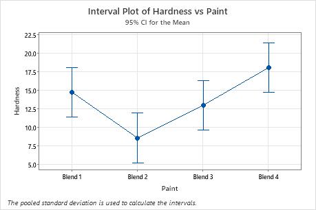
In the interval plot, Blend 2 has the lowest mean and Blend 4 has the highest. You cannot determine from this graph whether any differences are statistically significant. To determine statistical significance, assess the confidence intervals for the differences of means.
Step 3: Compare the group means
If your one-way ANOVA p-value is less than your significance level, you know that some of the group means are different, but not which pairs of groups. Use the grouping information table and tests for differences of means to determine whether the mean difference between specific pairs of groups are statistically significant and to estimate by how much they are different.
For more information on comparison methods, go to Using multiple comparisons to assess the practical and statistical significance.
- Grouping Information table
-
Use the grouping information table to quickly determine whether the mean difference between any pair of groups is statistically significant.
Groups that do not share a letter are significantly different.
- Tests for differences of means
-
Use the confidence intervals to determine likely ranges for the differences and to determine whether the differences are practically significant. The table displays a set of confidence intervals for the difference between pairs of means. The interval plot for differences of means displays the same information.
Confidence intervals that do not contain zero indicate a mean difference that is statistically significant.
Depending on the comparison method you chose, the table compares different pairs of groups and displays one of the following types of confidence intervals.-
Individual confidence level
The percentage of times that a single confidence interval includes the true difference between one pair of group means, if you repeat the study multiple times.
-
Simultaneous confidence level
The percentage of times that a set of confidence intervals includes the true differences for all group comparisons, if you repeat the study multiple times.
Controlling the simultaneous confidence level is particularly important when you perform multiple comparisons. If you do not control the simultaneous confidence level, the chance that at least one confidence interval does not contain the true difference increases with the number of comparisons.
-
For more information, go to Understanding individual and simultaneous confidence levels in multiple comparisons.
For more information about how to interpret the results for Hsu's MCB, go to What is Hsu's multiple comparisons with the best (MCB)?
Grouping Information Using the Tukey Method and 95% Confidence
| Paint | N | Mean | Grouping | |
|---|---|---|---|---|
| Blend 4 | 6 | 18.07 | A | |
| Blend 1 | 6 | 14.73 | A | B |
| Blend 3 | 6 | 12.98 | A | B |
| Blend 2 | 6 | 8.57 | B | |
Key Results: Mean, Grouping
In these results, the table shows that group A contains Blends 1, 3, and 4, and group B contains Blends 1, 2, and 3. Blends 1 and 3 are in both groups. Differences between means that share a letter are not statistically significant. Blends 2 and 4 do not share a letter, which indicates that Blend 4 has a significantly higher mean than Blend 2.
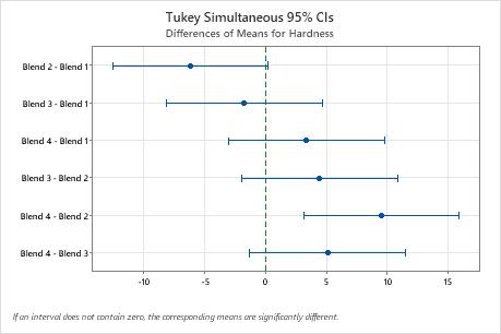
Tukey Simultaneous Tests for Differences of Means
| Difference of Levels | Difference of Means | SE of Difference | 95% CI | T-Value | Adjusted P-Value |
|---|---|---|---|---|---|
| Blend 2 - Blend 1 | -6.17 | 2.28 | (-12.55, 0.22) | -2.70 | 0.061 |
| Blend 3 - Blend 1 | -1.75 | 2.28 | (-8.14, 4.64) | -0.77 | 0.868 |
| Blend 4 - Blend 1 | 3.33 | 2.28 | (-3.05, 9.72) | 1.46 | 0.478 |
| Blend 3 - Blend 2 | 4.42 | 2.28 | (-1.97, 10.80) | 1.94 | 0.245 |
| Blend 4 - Blend 2 | 9.50 | 2.28 | (3.11, 15.89) | 4.17 | 0.002 |
| Blend 4 - Blend 3 | 5.08 | 2.28 | (-1.30, 11.47) | 2.23 | 0.150 |
Key Results: Simultaneous 95% CIs, Individual confidence level
- The confidence interval for the difference between the means of Blend 2 and 4 is 3.11 to 15.89. This range does not include zero, which indicates that the difference is statistically significant.
- The confidence intervals for the remaining pairs of means all include zero, which indicates that the differences are not statistically significant.
- The 95% simultaneous confidence level indicates that you can be 95% confident that all the confidence intervals contain the true differences.
- The table indicates that the individual confidence level is 98.89%. This result indicates that you can be 98.89% confident that each individual interval contains the true difference between a specific pair of group means. The individual confidence levels for each comparison produce the 95% simultaneous confidence level for all six comparisons.
Step 4: Determine how well the model fits your data
To determine how well the model fits your data, examine the goodness-of-fit statistics in the Model Summary table.
- S
- Use S to assess how well the model describes the response.
S is measured in the units of the response variable and represents how far the data values fall from the fitted values. The lower the value of S, the better the model describes the response. However, a low S value by itself does not indicate that the model meets the model assumptions. You should check the residual plots to verify the assumptions.
- R-sq
-
R2 is the percentage of variation in the response that is explained by the model. The higher the R2 value, the better the model fits your data. R2 is always between 0% and 100%.
A high R2 value does not indicate that the model meets the model assumptions. You should check the residual plots to verify the assumptions.
- R-sq (pred)
-
Use predicted R2 to determine how well your model predicts the response for new observations. Models that have larger predicted R2 values have better predictive ability.
A predicted R2 that is substantially less than R2 may indicate that the model is over-fit. An over-fit model occurs when you add terms for effects that are not important in the population. The model becomes tailored to the sample data and, therefore, may not be useful for making predictions about the population.
Predicted R2 can also be more useful than adjusted R2 for comparing models because it is calculated with observations that are not included in the model calculation.
Model Summary
| S | R-sq | R-sq(adj) | R-sq(pred) |
|---|---|---|---|
| 3.95012 | 47.44% | 39.56% | 24.32% |
Key Results: S, R-sq, R-sq (pred)
In these results, the factor explains 47.44% of the variation in the response. S indicates that the standard deviation between the data points and the fitted values is approximately 3.95 units.
Step 5: Determine whether your model meets the assumptions of the analysis
Use the residual plots to help you determine whether the model is adequate and meets the assumptions of the analysis. If the assumptions are not met, the model may not fit the data well and you should use caution when you interpret the results.
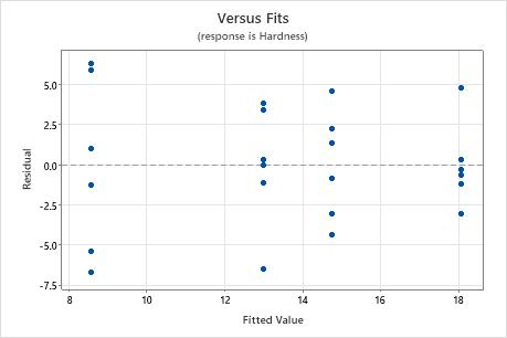
Residuals versus fits plot
Use the residuals versus fits plot to verify the assumption that the residuals are randomly distributed and have constant variance. Ideally, the points should fall randomly on both sides of 0, with no recognizable patterns in the points.
| Pattern | What the pattern may indicate |
|---|---|
| Fanning or uneven spreading of residuals across fitted values | Nonconstant variance |
| A point that is far away from zero | An outlier |
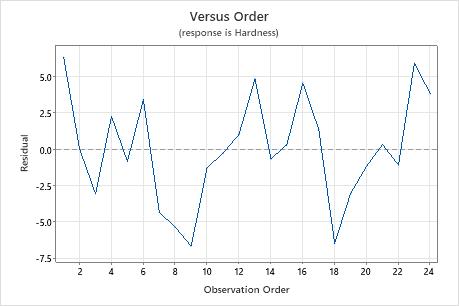
Residuals versus order plot
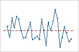
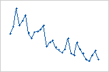
Trend
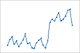
Shift
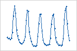
Cycle
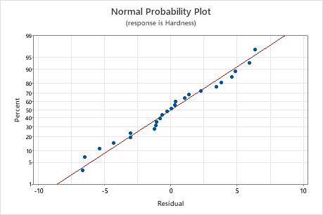
Normal probability plot of the residuals
Use the normal probability plot of the residuals to verify the assumption that the residuals are normally distributed. The normal probability plot of the residuals should approximately follow a straight line.
| Pattern | What the pattern may indicate |
|---|---|
| Not a straight line | Nonnormality |
| A point that is far away from the line | An outlier |
| Changing slope | An unidentified variable |
Note
If your one-way ANOVA design meets the guidelines for sample size, the results are not substantially affected by departures from normality.