In This Topic
Tolerance interval methods
Minitab calculates both parametric and nonparametric tolerance intervals. The calculations for the parametric tolerance intervals assume that the parent distribution of the sample is normally distributed. The calculations for the nonparametric tolerance intervals assume only that the parent distribution is continuous.
General Definitions
Let X 1, X 2, ..., X n be the ordered statistics based on random sample of size n from some continuous distribution.
Let the distribution function be F(x;θ) for Ω in some parameter space with dimension greater than or equal to 1.
Let L < U be two statistics based on the sample such that for any given values α and P, with 0 < α < 1 and 0 < P < 1, the following holds for every θ in Ω:

Then, the interval [L, U] is a two-sided tolerance interval with content = P x 100% and confidence level = 100(1 – α)%. Such an interval can be called a two-sided (1 – α, P) tolerance interval. For example, if α = 0.10 and P = 0.85, then the resulting interval is called a two-sided (90% , 0.85) tolerance interval.
If L = –∞ and U < +∞, then the interval (-∞, U] is called a one-sided (1 – α, P) upper tolerance bound. If L > -∞ and U = +∞, then the interval [L, +∞) is called a one-sided (1 – α, P) lower tolerance bound.
- A one-sided (1 – α, P) lower tolerance bound is also a one-sided (α, 1 – P) upper tolerance bound.
- A one-sided (1 – α )100% lower confidence bound of the (1 – P)th percentile of the distribution of the data is also a one-sided (1 – α, P) lower tolerance bound. Similarly, a one-sided (1 – α )100% upper confidence bound of the P th percentile of the distribution of the data is also a one-sided (1 – α , P) upper tolerance bound.
- If L and U are one-sided (1 – α/2 , (1 + P )/2) lower and upper tolerance bounds, then [ L, U ] is an approximate two-sided (1 – α, P ) tolerance interval. This method may be used in cases where two-sided tolerance intervals cannot be directly obtained. The resulting two-sided tolerance intervals are generally conservative. See Guenther1 and Hahn and Meeker2.
- Guenther, W. C. (1972). Tolerance intervals for univariate distributions. Naval Research Logistics, 19: 309–333.
- Hahn G. J. and Meeker W. Q. (1991). Statistical Intervals: A Guide for Practitioners John Wiley & Sons, New York.
Exact tolerance intervals for normal distributions


Tolerance factor for one-sided intervals
The exact tolerance factor for a one-sided interval is given by the following equation: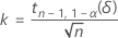
where tn-1,1-α(δ) is the 1 – α percentile of the noncentral t-distribution with n – 1 degrees of freedom and noncentrality parameter, δ, which is given by the following formula:

Tolerance factor for two-sided intervals
The exact tolerance factor for a two-sided interval is obtained by solving the following equation for k. See Krishnamoorthy and Mathew1.
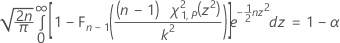
where Fn – 1 is the cumulative distribution function for a chi-square distribution with n – 1 degrees of freedom, and χ21,p is the Pth percentile of the noncentral chi-square distribution with 1 degree of freedom and noncentrality parameter z2. The left-hand side of the equation can be rewritten as:
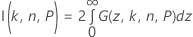
where:
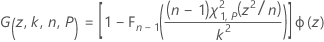
where Φ(z) is the probability density function of the standard normal distribution. Minitab uses a 36-point Gauss-Legendre quadrature to evaluate I(k, n, P).
Notation
| Term | Description |
|---|---|
| 1 - α | the confidence level of the tolerance interval |
| P | the coverage of the tolerance interval (the target minimum percentage of population in the interval) |
| L | the lower limit of the tolerance interval |
| U | the upper limit of the tolerance interval |
 | the mean of the sample |
| k | the tolerance factor (also called k-factor) |
| S | the standard deviation of the sample |
| n | the number of observations in the sample |
| ZP | the Pth percentile of the standard normal distribution |
- Krishnamoorthy, K. and Mathew, T. (2009). Statistical Tolerance Regions: Theory, Applications, and Computation. Wiley, Hoboken, NJ.
Exact nonparametric tolerance intervals for continuous distributions
Minitab calculates exact (1 – α, P) nonparametric tolerance intervals, where 1 – α is the confidence level and P is the coverage (the target minimum percentage of population in the interval). The nonparametric method for tolerance intervals is a distribution free method. That is, the nonparametric tolerance interval does not depend on the parent population of your sample. Minitab uses an exact method for both one-sided and two-sided intervals.
Let X 1, X 2 , ... , X n be the ordered statistics based on a random sample from some continuously distributed population F(x;θ). Then, based on the findings of Wilks1, 2 and Robbins3, it can be shown that:

where B denotes the cumulative distribution function of the beta distribution with parameters a = r and b = n – s + 1. Thus ( Xr , Xs ) is a distribution-free tolerance interval because the coverage of the interval has a beta distribution with known parameter values, which are independent of the distribution of the parent population, F(x;θ).
One-sided intervals
Let k be the largest integer that satisfies the following:

where Y is a binomial random variable with parameters n and 1 – P. It can be shown (see Krishnamoorthy and Mathew4) that a one-sided (1 – α, P) lower tolerance bound is given by Xk . Similarly, a one-sided (1 – α, P) upper tolerance bound is given by X n - k +1. In both cases, the actual or effective coverage is given by P(Y > k).
Two-sided intervals
Let k be the smallest integer that satisfies the following:

where V is a binomial random variable with parameters n and P. Thus,
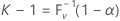
where F V -1(x) is the inverse cumulative distribution function of V. It can be shown (see Krishnamoorthy and Mathew4) that a two-sided (1 – α, P) tolerance interval may be given as ( Xr , Xs ). Minitab chooses s = n - r + 1 so that r = ( n – k + 1) / 2. Both r and s are rounded down to the nearest integer. The actual or effective coverage is given by P(V < k – 1).
Notation
| Term | Description |
|---|---|
| 1 – α | the confidence level of the tolerance interval |
| P | the coverage of the tolerance interval (the target minimum percentage of population in the interval) |
| n | the number of observations in the sample |
- Wilks, S. S. (1941). Sample size for tolerance limits on a normal distribution. The Annals of Mathematical Statistics, 12, 91–96.
- Wilks, S. S. (1941). Statistical prediction with special reference to the problem of tolerance limits. The Annals of Mathematical Statistics, 13, 400–409.
- Robbins, H. (1944). On distribution-free tolerance limits in random sampling. The Annals of Mathematical Statistics, 15, 214–216.
- Krishnamoorthy, K. and Mathew, T. (2009). Statistical Tolerance Regions: Theory, Applications, and Computation. Wiley, Hoboken, NJ.