In This Topic
Probability plot
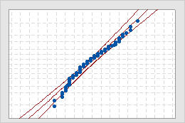
- Middle line
- The expected percentile from the distribution based on maximum likelihood parameter estimates.
- Confidence bound lines
- A left curved line indicates the lower bounds of the confidence intervals for the percentiles. A right curved line indicates the upper bounds of the confidence intervals for the percentiles.
Interpretation
Use the probability plot to assess how closely your data follow each distribution.
If the distribution is a good fit for the data, the points should fall closely along the fitted distribution line. Departures from the straight line indicate that the fit is unacceptable.
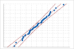
Good fit
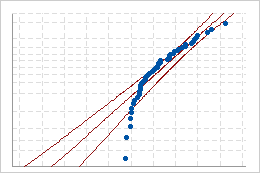
Poor fit
In addition to the probability plot, use the goodness-of-fit measures, such as the AD p-values and the LRT p-values, to evaluate the distribution fit.
- Choose the distribution that is most commonly used in your industry or application.
- Choose the distribution that provides the most conservative results. For example, if you are performing capability analysis, you can perform the analysis using different distributions and then choose the distribution that produces the most conservative capability indices. For more information, go to Distribution percentiles for Individual Distribution Identification and click "Percents and percentiles".
- Choose the simplest distribution that fits your data well. For example, if a 2-parameter and a 3-parameter distribution both provide a good fit, you might choose the simpler 2-parameter distribution.
AD
The Anderson-Darling goodness-of-fit statistic (AD) is a measure of the deviations between the fitted line (based on the selected distribution) and the nonparametric step function (based on the data points). The Anderson-Darling statistic is a squared distance that is weighted more heavily in the tails of the distribution.
Interpretation
Minitab uses the Anderson-Darling statistic to calculate the p-value. The p-value is a probability that measures the evidence against the null hypothesis that the data follow the distribution.
Generally, substantially smaller values for the Anderson-Darling statistic indicate that the data follow a distribution more closely. However, avoid directly comparing AD values across different distributions when the AD values are close, because AD statistics are distributed differently for different distributions. To better compare the fit of different distributions, use additional criteria, such as the probability plots, the p-values, and your process knowledge.
P
Note
No p-value for the AD test is available for the 3-parameter distributions, except for the Weibull distribution.
Interpretation
Use the p-value to assess the fit of the distribution.
- P ≤ α: The data do not follow the distribution (Reject H0)
- If the p-value is less than or equal to the significance level, the decision is to reject the null hypothesis and conclude that your data do not follow the distribution.
- P > α: Cannot conclude the data do not follow the distribution (Fail to reject H0)
- If the p-value is greater than the significance level, the decision is to fail to reject the null hypothesis. There is not enough evidence to conclude that the data do not follow the distribution. You can assume the data follow the distribution.
- Choose the distribution that is most commonly used in your industry or application.
- Choose the distribution that provides the most conservative results. For example, if you are performing capability analysis, you can perform the analysis using different distributions and then choose the distribution that produces the most conservative capability indices. For more information, go to Distribution percentiles for Individual Distribution Identification and click "Percents and percentiles".
- Choose the simplest distribution that fits your data well. For example, if a 2-parameter and a 3-parameter distribution both provide a good fit, you might choose the simpler 2-parameter distribution.
Important
Use caution when you interpret results from a very small or a very large sample. If you have a very small sample, a goodness-of-fit test may not have enough power to detect significant deviations from the distribution. If you have a very large sample, the test may be so powerful that it detects even small deviations from the distribution that have no practical significance. Use the probability plots in addition to the p-values to evaluate the distribution fit.
Goodness of Fit Test
| Distribution | AD | P | LRT P |
|---|---|---|---|
| Normal | 0.754 | 0.046 | |
| Box-Cox Transformation | 0.414 | 0.324 | |
| Lognormal | 0.650 | 0.085 | |
| 3-Parameter Lognormal | 0.341 | * | 0.017 |
| Exponential | 20.614 | <0.003 | |
| 2-Parameter Exponential | 1.684 | 0.014 | 0.000 |
| Weibull | 1.442 | <0.010 | |
| 3-Parameter Weibull | 0.230 | >0.500 | 0.000 |
| Smallest Extreme Value | 1.656 | <0.010 | |
| Largest Extreme Value | 0.394 | >0.250 | |
| Gamma | 0.702 | 0.071 | |
| 3-Parameter Gamma | 0.268 | * | 0.006 |
| Logistic | 0.726 | 0.034 | |
| Loglogistic | 0.659 | 0.050 | |
| 3-Parameter Loglogistic | 0.432 | * | 0.027 |
| Johnson Transformation | 0.124 | 0.986 |
In these results, several distributions have a p-value greater than 0.05. The 3-parameter Weibull distribution (P > 0.500) and the largest extreme value distribution (P > 0.250) have the largest p-values, and appear to fit the sample data better than the other distributions. Also, the Box-Cox transformation (P = 0.324) and the Johnson transformation (P = 0.986) are effective in transforming the data to follow a normal distribution.
Note
For several distributions, Minitab also displays results for the distribution with an additional parameter. For example, for the lognormal distribution, Minitab displays results for both the 2-parameter and 3-parameter versions of the distribution. For distributions that have additional parameters, use the likelihood-ratio test p-value (LRT P) to determine whether adding another parameter significantly improves the fit of the distribution. An LRT p-value that is less than 0.05 suggests that the improvement in fit is significant. For more information, see the section on LRT P.
LRT P
For several distributions, Minitab also displays results for the distribution with an additional parameter. For each extra-parameter version of a distribution, Minitab reports a p-value for the likelihood-ratio test (LRT P). A p-value is a probability that measures the evidence against the null hypothesis. For the likelihood-ratio test in individual distribution identification, the null hypothesis is that the data follow the smaller (lower parameter) distribution. Therefore, lower LRT p-values provide stronger evidence that the distribution fit is significantly improved by using an additional parameter.
Interpretation
Use the LRT p-value to determine whether adding the extra parameter significantly improves the fit over the distribution without the extra parameter.
- P ≤ α: The larger (higher parameter) distribution provides a significantly better fit. (Reject H0)
- If the p-value is less than or equal to the significance level, you reject the null hypothesis and conclude that the distribution fit is significantly improved by using an additional parameter.
- P > α: Cannot conclude that the larger (higher parameter) distribution provides a significantly better fit (Fail to reject H0)
- If the p-value is greater than the significance level, you fail to reject the null hypothesis. There is not enough evidence to conclude that the distribution fit is significantly improved by using an additional parameter.
The LRT p-value is also useful for 3-parameter distributions for which there is no established method for calculating the p-value. In these cases, first examine the p-value for the corresponding 2-parameter distribution. Then examine the LRT p-value for the 3-parameter distribution to determine whether the 3-parameter distribution is significantly better than the 2-parameter distribution.
In these results, the LRT p-values for the 3-parameter lognormal (0.017), 3-parameter Weibull (0.000), 3-parameter gamma (0.006), and 3-parameter loglogistic (0.027) distributions suggest that these distributions significantly improve the fit compared to their 2-parameter counterparts.
Goodness of Fit Test
| Distribution | AD | P | LRT P |
|---|---|---|---|
| Normal | 0.754 | 0.046 | |
| Box-Cox Transformation | 0.414 | 0.324 | |
| Lognormal | 0.650 | 0.085 | |
| 3-Parameter Lognormal | 0.341 | * | 0.017 |
| Exponential | 20.614 | <0.003 | |
| 2-Parameter Exponential | 1.684 | 0.014 | 0.000 |
| Weibull | 1.442 | <0.010 | |
| 3-Parameter Weibull | 0.230 | >0.500 | 0.000 |
| Smallest Extreme Value | 1.656 | <0.010 | |
| Largest Extreme Value | 0.394 | >0.250 | |
| Gamma | 0.702 | 0.071 | |
| 3-Parameter Gamma | 0.268 | * | 0.006 |
| Logistic | 0.726 | 0.034 | |
| Loglogistic | 0.659 | 0.050 | |
| 3-Parameter Loglogistic | 0.432 | * | 0.027 |
| Johnson Transformation | 0.124 | 0.986 |