Example of using ICDF to determine warranty periods
For example, an appliance manufacturer investigates failure times for the heating element within its toasters. They want to determine the time by which specific proportions of heating elements will fail so they can set the warranty period. Heating element failure times follow a normal distribution with a mean of 1000 hours and standard deviation of 300 hours. The probability density function (PDF) helps identify regions of higher and lower failure probabilities. The inverse CDF gives the corresponding failure time for each cumulative probability.
Use the inverse CDF to estimate the time by which 5% of the heating elements will fail, times between which 95% of all heating elements will fail, or the time at which only 5% of the heating elements remain. The inverse CDF for specific cumulative probabilities is equal to the failure time at the right side of the shaded area under the PDF curve.
Determine the time at which 5% will fail
- Choose .
- Choose Inverse cumulative probability. In Mean, enter 1000. In Standard deviation, enter 300. In Input constant, enter 0.05.
- Click OK.
The time by which 5% of the heating elements are expected to have failed is the inverse CDF of 0.05 or 506.544 hours.
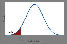
This plot illustrates the inverse CDF.
Determine times between which 95% will fail
- Choose .
-
Choose
Inverse cumulative probability.
In
Mean,
enter
1000. In
Standard deviation,
enter
300. In
Input constant,
enter
0.025. Click
OK.
The time by which 2.5% of the heating elements are expected to have failed is the inverse CDF of 0.025 or 412 hours.
-
Repeat step 2, but enter
0.975 instead of
0.025. Click
OK.
The time by which 97.5% of the heating elements are expected to have failed is the inverse CDF of 0.975 or 1588 hours.
Therefore, times between which 95% of all heating elements are expected to fail is the inverse CDF of 0.025 and the inverse CDF of 0.975 or 412 hours and 1588 hours.
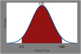
This plot illustrates the inverse CDF.
Determine the time at which 5% will survive
- Choose .
- Choose Inverse cumulative probability. In Mean, enter 1000. In Standard deviation, enter 300. In Input constant, enter 0.95.
- Click OK.
The time at which only 5% of the heating elements are expected to remain is the inverse CDF of 0.95 or 1493 hours.
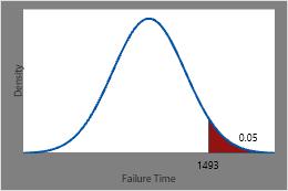
This plot illustrates the inverse CDF.
Example of using the CDF and the ICDF with the hypergeometric distribution
When you try to determine the inverse cumulative probability of a discrete distribution, the output in contains two sets of columns.
Suppose you have the inverse cumulative probability of a proportion, p. The first set of columns in the output lists the largest x such that P(X ≤ x) ≤ p. The second set of columns lists the smallest x such that P(X ≤ x) ≥ p.
Calculate the cumulative probability of a hypergeometric distribution
-
In worksheet column C1, enter
0 1 2.
C1 0 1 2 - Choose .
- Choose Cumulative probability.
- In Population size (N), type 20000.
- In Event count in population (M), type 2000.
- In Sample size (n), type 20.
- Choose Input column and enter C1. Click OK.
Cumulative Distribution Function
- P(X ≤ 0) = 0.121448. The probability of getting 0 defects is about 12%.
- P(X ≤ 1) = 0.391619. The probability of getting 0 or 1 defects is about 39%.
- P(X ≤ 2) = 0.676941. The probability of getting 0, 1, or 2 defects is about 68%.
Calculate the inverse cumulative probability of a hypergeometric distribution
Now that you know the cumulative probabilities associated with the number of defects, calculate the inverse cumulative probability.
Suppose that you want to calculate the number of defects, x, such that the cumulative probability, p, is 0.50. From the previous results, you know that P(X ≤ 1 ) = 0.391619 and P(X ≤ 2 ) = 0.676941. Because the hypergeometric distribution is a discrete distribution, the number of defects cannot be between 1 and 2. In other words, you may have 1 defect or 2 defects, but not 1.4 defects. Therefore, if you choose Input constant and enter 0.50, Minitab calculates both probabilities in the output, as shown in the following example:
- Choose .
- Choose Inverse cumulative probability.
- In Population size (N), type 20000.
- In Event count in population (M), type 2000.
- In Sample size (n), type 20.
- Choose Input constant, and type 0.50. Click OK.
Inverse Cumulative Distribution Function
The first probability indicates a value of x such that P(X ≤ x) < p and the second probability indicates the smallest x such that P(X ≤ x) ≥ p. In this example, the first probability shows the largest number of defectives, x = 2, such that P(X ≤ 2) <0.5 and the 2nd shows the smallest number of defectives, x = 3, such that P(X ≤ 3) ≥ 0.5.
Use the ICDF to calculate critical values
You can use Minitab to calculate a critical value for a hypothesis test instead of looking in a table.
Suppose that you perform a chi-square test with an α = 0.02 and 12 degrees of freedom. What is the corresponding critical value? An α = 0.02 corresponds to a cumulative probability value of 1 – 0.02 = 0.98.
- Choose .
- Choose Inverse cumulative probability.
- In Degrees of freedom, enter 12.
- Choose Input constant and enter 0.98.
- Click OK.
Minitab displays the critical value, 24.054. For the chi-square test, if the test statistic is greater than the critical value, you can conclude that there is statistical evidence to reject the null hypothesis.
Note
This example uses the chi-square distribution. However, you follow these same steps for any distribution that you select.