In This Topic
Significance level (α)
The significance level (denoted by alpha or α) is the maximum acceptable level of risk for a type I error.
Interpretation
Use the significance level to decide whether an effect is statistically significant. Because the significance level is the threshold for statistical significance, a higher value increases the chance of making a type I error. A type I error is the incorrect conclusion that an effect is statistically significant.
Assumed standard deviation
The assumed standard deviation is the estimate of the standard deviation of the response measurements at replicated experimental runs. If you already performed an analysis in minitab that produced an ANOVA table, you can use the square root of the adjusted mean square for error.
Interpretation
Use the assumed standard deviation to describe how variable the data are. Higher values of the assumed standard deviation indicate more variation or "noise" in the data, which decreases the statistical power of a design.
Factors
The number shows how many factors are in the design.
Interpretation
Use the number of factors to verify that the design has all of the factors that you need to study. Factors are the variables that you control in the experiment. Factors are also known as independent variables, explanatory variables, and predictor variables. For the power and sample size calculations, all factors are numeric. Numeric factors use a few controlled values in the experiment, even though many values are possible. These values are known as factor levels.
For example, you are studying factors that could affect plastic strength during the manufacturing process. You decide to include Temperature in your experiment. Because temperature is a factor, only three temperatures settings are in the experiment: 100 °C, 150 °C, and 200 °C.
Base design
The numbers show the number of factors and the number of corner points in the base design.
Interpretation
Use the base design to determine whether the experimental design is a full design or a fractional design. If the number of corner points is less than 2^(number of factors), then the experimental design is a fractional design. In a fractional design, not all of the terms the design can estimate are independent of each other. To see how the terms depend on each other, create the design and review the alias table.
The base design is the starting point from which you can build your final design. You can add to the base design to achieve different purposes. For example, you can add replicates or center points to increase the power of the design.
Blocks
The number shows how many blocks are in the design.
Interpretation
Use the number of blocks to identify the design that the power calculations use. Blocks are groups of experimental runs conducted under relatively homogeneous conditions. Although every measurement should be taken under consistent experimental conditions (other than those that are being varied as part of the experiment), this is not always possible.
For example, you want to test the quality of a new printing press. However, press setup takes several hours and can only be done four times a day. Because the design of the experiment requires at least eight runs, you need at least two days to test the press. You should account for any differences in conditions between days by using "day" as a blocking variable. To distinguish between any block effect (incidental differences between days) and effects due to the experimental factors (temperature, humidity, and press operator), you must account for the block (day) in the experimental design. You should randomize run order within blocks. For more information on how Minitab assigns runs to blocks, go to What is a block?
Center points per block
The number shows how many center points per block are in the design.
Interpretation
Use the number of center points per block to identify the design that the power calculations use. Center points are runs where all of the factors are set midway between their low and high levels. If the design includes blocks, then Minitab adds the same number of center points to each block. For example, if you specify 2 center points per block and 2 blocks, the design includes 4 center points.
Center points usually have a small influence on the results when the design includes replicates of the corner points. Center points have other uses besides their influence on the power calculations. For example, the test for curvature in the response requires center points.
In these results, the points on the power curves show calculations for a difference of 2.5. The design with 1 replicate and no center points has a power close to 0.56. The design with 1 replicate and 6 center points has a power of almost 0.7. With two replicates, the power curves for 0 center points and 6 center points are indistinguishable on the graph. The curve for 6 center points is slightly higher for nonzero effects. The power values are both over 0.95.
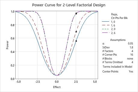
Method
| Factors: | 4 | Base Design: | 4, 16 |
|---|---|---|---|
| Blocks: | none |
Results
| Center Points | Effect | Reps | Total Runs | Power |
|---|---|---|---|---|
| 0 | 2.5 | 1 | 16 | 0.557255 |
| 0 | 2.5 | 2 | 32 | 0.961939 |
| 6 | 2.5 | 1 | 22 | 0.696490 |
| 6 | 2.5 | 2 | 38 | 0.965121 |
Effect
If you enter the number of replicates, the power value, and the number of center points, Minitab calculates the effect. The effect is the difference in the response between the high and low levels of a factor that you want the design to detect. This difference is the result of one factor alone (main effect).
Interpretation
Use the effect size to determine the ability of the design to detect an effect. If you enter a number of replicates, a power, and a number of center points, then Minitab calculates the smallest effect size that the design can detect with the specified power. Usually, more replicates allow a designed experiment to detect smaller effects.
In these results, the design with one replicate can detect a difference of about 0.015 with 80% power. The difference that the design can detect with 90% power is larger than 0.015, about 0.018. The design with 2 replicates can detect a difference that is smaller than 0.015 with 80% power, about 0.007.
Method
| Factors: | 5 | Base Design: | 5, 32 |
|---|---|---|---|
| Blocks: | none |
Results
| Center Points | Reps | Total Runs | Power | Effect |
|---|---|---|---|---|
| 4 | 1 | 36 | 0.8 | 0.0153027 |
| 4 | 1 | 36 | 0.9 | 0.0180278 |
| 4 | 2 | 68 | 0.8 | 0.0073261 |
| 4 | 2 | 68 | 0.9 | 0.0084775 |
Reps
Replicates are multiple experimental runs with the same factor settings.
Interpretation
Use the number of replicates to estimate how many experimental runs to include in the design. If you enter a power, effect size, and number of center points, Minitab calculates the number of replicates. Because the numbers of replicates and center points are given in integer values, the actual power may be greater than your target value. If you increase the number of replicates, the power of your design also increases. You want enough replicates to achieve adequate power.
Because the replicates are integer values, the power values that you specify are target power values. The actual power values are for the number of replicates and the number of center points in the designed experiment. The actual power values are at least as large as the target power values.
In these results, Minitab calculates the number of replicates to reach the target power. The design that detects an effect of 2 with a power of 0.8 requires 1 replicate. To achieve a power of 0.9, the design requires 2 replicates. The actual power with 2 replicates is greater than 0.99. This actual power is the smallest power value that is greater than or equal to 0.9 and obtainable using an integer number of replicates. To detect the smaller effect of 0.9 with 0.8 power, the design requires 4 replicates. To detect the smaller effect of 0.9 with 0.9 power, the design requires 5 replicates.
Method
| Factors: | 15 | Base Design: | 15, 32 |
|---|---|---|---|
| Blocks: | none |
Results
| Center Points | Effect | Reps | Total Runs | Target Power | Actual Power |
|---|---|---|---|---|---|
| 0 | 2.0 | 1 | 32 | 0.8 | 0.877445 |
| 0 | 2.0 | 2 | 64 | 0.9 | 0.995974 |
| 0 | 0.9 | 4 | 128 | 0.8 | 0.843529 |
| 0 | 0.9 | 5 | 160 | 0.9 | 0.914018 |
Compare the first set of results to the second set of results. In the first set of results, 16 terms are omitted from the model. In the second set of results, the model includes all estimable terms. Because the second model uses all degrees of freedom for a single replicate of the design, Minitab does not include 1 replicate as a solution. Because the number of terms in the model is higher, the other power values are lower than in the results where the model omits terms. For example, the actual power for the design with 5 replicates is about 0.9140 in the first set of results and about 0.9136 in the second set of results.
Method
| Factors: | 15 | Base Design: | 15, 32 |
|---|---|---|---|
| Blocks: | none |
Results
| Center Points | Effect | Reps | Total Runs | Target Power | Actual Power |
|---|---|---|---|---|---|
| 0 | 2.0 | 2 | 64 | 0.8 | 0.995347 |
| 0 | 2.0 | 2 | 64 | 0.9 | 0.995347 |
| 0 | 0.9 | 4 | 128 | 0.8 | 0.842492 |
| 0 | 0.9 | 5 | 160 | 0.9 | 0.913575 |
Total Runs
An experimental run is a factor level combination at which you measure responses. The total number of runs is how many measurements of the response are in the design. Multiple executions of the same factor level combination are considered separate experimental runs and are called replicates.
Interpretation
Use the number of total runs to verify that the designed experiment is the right size for your resources. For a 2-level factorial design, this formula gives the total number of experimental runs:

| Term | Description |
|---|---|
| n | Number of replicates |
| r | Number of corner points per replicate |
| cpblock | Number of center points per block |
| b | Number of blocks |
In these results, the base design has 16 corner points. The design has 4 blocks and 4 center points per block, for a total of 4*4 = 16 center points. So the design with 1 replicate has 16 corner points and 16 center points for a total of 16 + 16 = 32 experimental runs. The design with 2 replicates doubles the number of corner points to 2*16 = 32. The number of blocks and the number of center points per block remains the same. As a result, the design with 2 replicates has a total of 32 + 16 = 48 runs.
Method
| Factors: | 4 | Base Design: | 4, 16 |
|---|---|---|---|
| Blocks: | 4 |
Results
| Center Points Per Block | Effect | Reps | Total Runs | Power |
|---|---|---|---|---|
| 4 | 2.5 | 1 | 32 | 0.741569 |
| 4 | 2.5 | 2 | 48 | 0.967699 |
Power
The power of a design is the probability that the design determines that an effect is statistically significant. The difference between the means of the response variable at the high and low levels of a factor is the effect size.
Interpretation
Use the power value to determine the ability of the design to detect an effect. If you enter a number of replicates, an effect size, and a number of center points, then Minitab calculates the power of the design. A power value of 0.9 is usually considered adequate. A value of 0.9 indicates that a design has a 90% chance to detect an effect of the size that you specify. Usually, the fewer the number of replicates, the lower the power. If a design has low power, you might fail to detect an effect and mistakenly conclude that none exists.
These results demonstrate how an increase in the number of experimental runs increases the power. For an effect size of 0.9, the power of the design is approximately 0.55 with 64 total runs. With 160 total runs the power of the design increases to about 0.91.
These results also demonstrate how an increase in the effect size increases the power. For a 64-run design, the power is approximately 0.55 for an effect size of 0.9. With an effect size of 1.5, the power increases to about 0.93.
Method
| Factors: | 15 | Base Design: | 15, 32 |
|---|---|---|---|
| Blocks: | none |
Results
| Center Points | Effect | Reps | Total Runs | Power |
|---|---|---|---|---|
| 0 | 1.5 | 5 | 160 | 0.999830 |
| 0 | 1.5 | 2 | 64 | 0.932932 |
| 0 | 0.9 | 5 | 160 | 0.914018 |
| 0 | 0.9 | 2 | 64 | 0.545887 |
Power curve
The power curve plots the power of the design versus the size of the effect. Effect refers to the difference between the mean response value at the high and low levels of a factor.
Interpretation
Use the power curve to assess the appropriate properties for your design.
The power curve represents the relationship between power and effect size, for every combination of center points and replicates. Each symbol on the power curve represents a calculated value based on the properties that you enter. For example, if you enter a number of replicates, a power value, and a number of center points, then Minitab calculates the corresponding effect size and displays the calculated value on the graph for the combination of replicates and center points. If you solve for replicates or center points, the plot also includes curves for other combinations of replicates and center points that are in the combinations that achieve the target power. The plot does not show curves for cases that do not have enough degrees of freedom to assess statistical significance.
Examine the values on the curve to determine the effect size that the experiment detects at a certain power value, number of corner points, and number of center points. A power value of 0.9 is usually considered adequate. However, some practitioners consider a power value of 0.8 to be adequate. If a design has low power, you might fail to detect an effect that is practically significant. Increasing the number of replicates increases the power of your design. You want enough experimental runs in your design to achieve adequate power. A design has more power to detect a larger effect than a smaller effect.
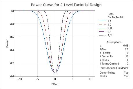
In these results, Minitab calculates the number of replicates to achieve a target power of at least 0.8 or 0.9 for an effect size of 3.5. The designed experiment has 16 corner points in 4 blocks to study 4 factors. The calculations consider designed experiments with 0, 1, or 2 center points per block. The curve that shows 1 replicate and two center points has a symbol for the effect of 3.5 where the power is higher than the target power of 0.8. The three curves that represent the experiments with 2 replicates have symbols that show that the power to detect an effect of 3.5 exceeds the target power of 0.9.
Because a solution exists with 2 replicates and 1 center point and a solution exists with 1 replicate and 2 center points, the plot also includes a curve for an experiment with 1 replicate and 1 center point. This experiment does not achieve either target power for the effect of 3.5, so this curve does not have a symbol. The plot does not include the symbol with 1 replicate and 0 center points because this experiment does not have enough degrees of freedom to assess statistical significance when 0 terms are omitted from the model.