Select the statistics to include in your output. Changes made in this sub-dialog box affect the current session only. To change the default settings for future sessions, choose . Select the desired statistics and click OK.
Note
Changing the default will not retroactively alter preferences for projects in which you have already run Display Descriptive Statistics. To change the statistics that are displayed with Display Descriptive Statistics in these projects, check the desired statistics in the Statistics sub-dialog box.
Mean
Use the mean to describe the sample with a single value that represents the center of the data. Many statistical analyses use the mean as a standard measure of the center of the distribution of the data.
SE of mean
Use the standard error of the mean to determine how precisely the mean of the sample estimates the population mean. For more information, go to All statistics and graphs and click "SE Mean".
Standard deviation
Use the standard deviation to determine how spread out the data are from the mean. For more information, go to What is the standard deviation?.
Variance
Use the variance to determine how spread out the data are from the mean. The variance is equal to the standard deviation squared. For more information, go to What is the variance?.
Coefficient of variation
The coefficient of variation (denoted as COV) is a measure of spread that describes the variation in the data relative to the mean. The coefficient of variation is adjusted so that the values are on a unitless scale. Because of this adjustment, you can use the coefficient of variation instead of the standard deviation to compare the variation in data that have different units or that have very different means. For more information, go to All statistics and graphs and click "CoefVar".
Range
The range is the difference between the largest and smallest data values in the sample. The range represents the smallest interval that contains all the data values.
Sum
The sum is the total of all of the data values.
Minimum
The minimum is the smallest data value in the sample. Use the minimum to identify a possible outlier or a data entry mistake. One of the simplest ways to assess the spread of your data is to compare the minimum and maximum.
First quartile
25% of the data values in the sample are less than the first quartile value.
Median
The median is another measure of the center of the distribution of the data. The median is usually less influenced by outliers than the mean. Half the data values are greater than the median value, and half the data values are less than the median value.
Third quartile
25% of the data values in the sample are greater than the third quartile value.
Maximum
The maximum is the largest data value in the sample. Use the maximum to identify a possible outlier or a data entry mistake. One of the simplest ways to assess the spread of your data is to compare the minimum and maximum.
Interquartile range
The interquartile range (IQR) is the distance between the first quartile (Q1) and the third quartile (Q3). Use the interquartile range to describe the spread of the data. As the spread of the data increases, the IQR becomes larger.
Mode
Use the mode to describe an entire set of observations with a single value that represents the most common value in the sample. You can use the mode along with the mean and median to obtain an overall characterization of your data distribution.
N nonmissing
The number of non-missing values in the sample. Minitab displays this value in the output as N.
N missing
The number of missing values in the sample. The number of missing values refers to cells that contain the missing value symbol *. Minitab displays this value in the output as N*.
N total
The total number of observations in the column. Use to represent the sum of N missing and N nonmissing. Minitab displays this value in the output as Total Count.
Cumulative N
| Grade Level | Count | CumN | Calculation |
|---|---|---|---|
| 1 | 49 | 49 | 49 |
| 2 | 58 | 107 | 49 + 58 |
| 3 | 52 | 159 | 49 + 58 + 52 |
| 4 | 60 | 219 | 49 + 58 + 52 + 60 |
| 5 | 48 | 267 | 49 + 58 + 52 + 60 + 48 |
| 6 | 55 | 322 | 49 + 58 + 52 + 60 + 48 + 55 |
Percent
The percent represents the contribution of a category to the whole. Percent is calculated by dividing the frequency of that category by the total frequency and multiplying by 100. For example, if you inspect 400 parts and 21 of them are defective, the percent defective would be 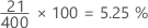 .
.
Cumulative percent
The cumulative percent is the sum of all the percentage values up to that category, as opposed to the individual percentages of each category.
Trimmed mean
Use the trimmed mean to eliminate the impact of very large or very small values on the mean. When the data contain outliers, the trimmed mean may be a better measure of central tendency than the mean.
Sum of squares
The uncorrected sum of squares are calculated by squaring each value in the column, and then adding those squared values. For example, if the column contains x1, x2, ... , xn, then the sum of squares is calculated as (x12 + x22 + ... + xn2). Unlike the corrected sum of squares, the uncorrected sum of squares includes error. The data values are squared without first subtracting the mean.
Skewness
Use skewness to determine the extent to which the data are not symmetrical. For more information, go to How skewness and kurtosis affect your distribution.
Kurtosis
Use kurtosis to determine the extent to which the data are peaked, compared to a normal curve. For more information, go to How skewness and kurtosis affect your distribution.
MSSD
The mean of the squared successive differences (MSSD) is an estimate of variance. One possible use of the MSSD is to test whether a sequence of observations is random. In quality control, a possible use of MSSD is to estimate the variance when the subgroup size = 1.