A quality engineer is concerned about two types of defects in molded resin parts: discoloration and clumping. Discolored streaks in the final product can result from contamination in hoses and from abrasions to resin pellets. Clumping can occur when the process is run at higher temperatures and faster rates of transfer. The engineer identifies three possible predictor variables for the responses (defects). The engineer records the number of each type of defect in hour long sessions, while varying the predictor levels.
The engineer wants to study how several predictors affect discoloration defects in resin parts. Because the response variable describes the number of times that an event occurs in a finite observation space, the engineer fits a Poisson model.
Choose Stat > Regression > Poisson Regression > Fit Poisson Model.
In Response, enter 'Discoloration Defects'.
In Continuous predictors, enter 'Hours Since Cleanse' Temperature.
In Categorical predictors, enter 'Size of Screw'.
Click Graphs.
In Residuals for plots, select Standardized.
Under Residuals plots, select Four in one.
Click OK in each dialog box.
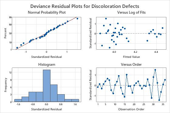
Interpret the results
The plot of the standardized deviance residuals versus the fitted values shows a distinct curve. In the plot of the residuals versus order, the residuals in the middle tend to be higher than the residuals at the beginning and end of the data set. For these data, both patterns are because of a missing interaction term between the size of the screw and the temperature. The pattern is visible on the residuals versus order plot because the engineer did not collect the data in random order. The engineer refits the model with the interaction between temperature and the size of the screw to model the defects more accurately.
Syntax Error
Regression Equation
Discoloration Defects
=
exp(Y')
Size of Screw
large
Y'
=
4.398 + 0.01798 Hours Since Cleanse - 0.001974 Temperature
small
Y'
=
4.244 + 0.01798 Hours Since Cleanse - 0.001974 Temperature
Coefficients
Term
Coef
SE Coef
Z-Value
P-Value
VIF
Constant
4.3982
0.0628
70.02
0.000
Hours Since Cleanse
0.01798
0.00826
2.18
0.029
1.00
Temperature
-0.001974
0.000318
-6.20
0.000
1.00
Size of Screw
small
-0.1546
0.0427
-3.62
0.000
1.00
Model Summary
Deviance R-Sq
Deviance R-Sq(adj)
AIC
AICc
BIC
64.20%
60.80%
253.29
254.58
259.62
Goodness-of-Fit Tests
Test
DF
Estimate
Mean
Chi-Square
P-Value
Deviance
32
31.60722
0.98773
31.61
0.486
Pearson
32
31.26713
0.97710
31.27
0.503
Analysis of Variance
Wald Test
Source
DF
Chi-Square
P-Value
Regression
3
56.29
0.000
Hours Since Cleanse
1
4.74
0.029
Temperature
1
38.46
0.000
Size of Screw
1
13.09
0.000
Fits and Diagnostics for Unusual Observations
Obs
Discoloration Defects
Fit
Resid
Std Resid
33
43.00
58.18
-2.09
-2.18
R
Press
Ctrl+E, or click the Edit Last
Dialog button
on the Standard toolbar.
Click Model.
In Predictors, select Temperature and 'Size of Screw'.
Next to Interactions through order, choose 2 and click Add.
Click OK in each dialog box.
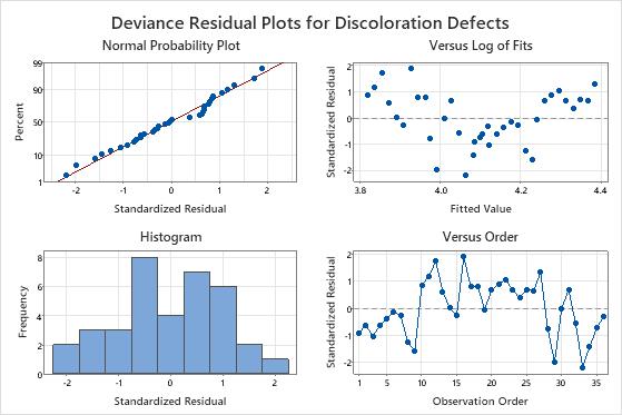
For the model with the interaction, the AIC is approximately 236, which is lower than the model without the interaction. The AIC criterion indicates that the model with the interaction is better than the model without the interaction. The curvature in the residuals versus fits plot is gone. The engineer notices that some coefficients have VIF values that are > 5. In this case, an analysis with standardized continuous predictors to reduce the effect of collinearity gives the same conclusions about the statistical significance of the terms in the model. (For more information, go to Multicollinearity in regression.) The engineer decides to interpret this model rather than the model without the interaction.
Method
Link function
Natural log
Categorical predictor coding
(1, 0)
Rows used
36
Regression Equation
Discoloration Defects
=
exp(Y')
Size of Screw
large
Y'
=
4.576 + 0.01798 Hours Since Cleanse - 0.003285 Temperature
small
Y'
=
4.032 + 0.01798 Hours Since Cleanse - 0.000481 Temperature
 on the Standard toolbar.