In This Topic
Fitted and predicted values
To calculate the prediction, invert the link function for the model. The inverse functions are in this table.
| Link Function | Formula for Prediction |
|---|---|
| Logit |  |
| Normit |  |
| Gompit | 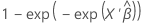 |
Notation
| Term | Description |
|---|---|
| exp(·) | the exponential function |
| Φ(·) | the cumulative distribution function of the normal distribution |
| X' | the transpose of the vector of points to predict for |
 | the vector of estimated coefficients |
Standard error of fitted values and predictions
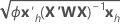
In general, the standard error of the fit has the following form:
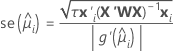
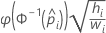
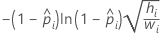
The following formulas give the standard error of the fit for different link functions:
- Logit

- Normit
- Gompit
Note the following relationship that applies to the formulas in the table: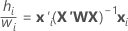
where  is from the training data only when there is a test data set for validation.
Notation
| Term | Description |
|---|---|
 | 1, for the binomial and Poisson models |
| xi | the vector of a design point |
 | the transpose of xi |
| X | the design matrix |
| W | the weight matrix |
 | the first derivative of the link function evaluated at  |
 | the predicted mean response |
 | the predicted probability for the design point in a binary logistic model |
 | the inverse cumulative distribution function of the standard normal distribution for the predicted probability in a binary logistic model |
 | the probability density function of the standard normal distribution |
Confidence limits for fits and predictions
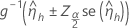
The confidence limits use the Wald approximation method. This is the formula for a 100(1 − α)% two-sided confidence interval:
Notation
| Term | Description |
|---|---|
 | the inverse of the link function evaluated at x |
 |  |
 | the transpose of the vector of the predictors |
 | the vector of estimated coefficients |
 | the value of the inverse cumulative distribution function for the normal distribution evaluated at  |
| α | the significance level |
 |  |
| X | the design matrix |
| W | the weight matrix |
 | 1, for binomial models |