In This Topic
Coefficients
[1] P. McCullagh and J. A. Nelder (1989). Generalized Linear Models, 2nd Ed., Chapman & Hall/CRC, London.
Standard error of coefficients

W is a diagonal matrix where the diagonal elements are given by the following formula:
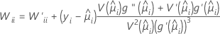
where

This variance-covariance matrix is based on the observed Hessian matrix as opposed to the Fisher's information matrix. Minitab uses the observed Hessian matrix because the model that results is more robust against any conditional mean misspecification.
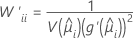
If the canonical link is used then the observed Hessian matrix and the Fisher's information matrix are identical.
Notation
| Term | Description |
|---|---|
| yi | the response value for the ith row |
 | the estimated mean response for the ith row |
| V(·) | the variance function given in the table below |
| g(·) | the link function |
| V '(·) | the first derivative of the variance function |
| g'(·) | the first derivative of the link function |
| g''(·) | the second derivative of the link function |

See [1] and [2] for more information.
[1] A. Agresti (1990). Categorical Data Analysis. John Wiley & Sons, Inc.
[2] P. McCullagh and J.A. Nelder (1992). Generalized Linear Model. Chapman & Hall.
Z
The Z-statistic used to determine whether the predictor is significantly related to the response. Larger absolute values of Z indicate a significant relationship. The formula is:

Notation
| Term | Description |
|---|---|
| Zi | The test statistic for a standard normal distribution |
 | The estimated coefficient |
 | The standard error of the estimated coefficient |
For small samples, the likelihood-ratio test may be a more reliable test of significance. The likelihood ratio p-values are in the deviance table. When the sample size is large enough, the p-values for the Z statistics approximate the p-values for the likelihood ratio statistics.
p-value (P)
Used in hypothesis tests to help you decide whether to reject or fail to reject a null hypothesis. The p-value is the probability of obtaining a test statistic that is at least as extreme as the actual calculated value, if the null hypothesis is true. A commonly used cut-off value for the p-value is 0.05. For example, if the calculated p-value of a test statistic is less than 0.05, you reject the null hypothesis.
Odds ratios for binary logistic regression
The odds ratio is provided only if you select the logit link function for a model with a binary response. In this case, the odds ratio is useful in interpreting the relationship between a predictor and a response.
The odds ratio (τ) can be any nonnegative number. The odds ratio = 1 serves as the baseline for comparison. If τ = 1, no association exists between the response and predictor. If τ < 1, the odds of the event are higher for the reference level of the factor (or for lower levels of a continuous predictor). If τ > 1, the odds of the event are less for the reference level of the factor (or for lower levels of a continuous predictor). Values farther from 1 represent stronger degrees of association.
Note
For the binary logistic regression model with one covariate or factor, the estimated odds of success are:
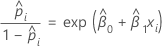
The exponential relationship provides an interpretation for β: The odds increase multiplicatively by eβ1 for every one-unit increase in x. The odds ratio is equivalent to exp(β1).
For example, if β is 0.75, the odds ratio is exp(0.75), which is 2.11. This indicates that there is a 111% increase in the odds of success for every one unit increase in x.
Notation
| Term | Description |
|---|---|
 | the estimated probability of a success for the ith row in the data |
 | the estimated intercept coefficient |
 | the estimated coefficient for predictor x |
 | the data point for the ith row |
Confidence interval
The large sample confidence interval for an estimated coefficient is:

For binary logistic regression, Minitab provides confidence intervals for the odds ratios. To obtain the confidence interval of the odds ratio, exponentiate the lower and upper limits of the confidence interval. The interval provides the range in which the odds may fall for every unit change in the predictor.
Notation
| Term | Description |
|---|---|
 | the ith coefficient |
 | the inverse cumulative probability of the standard normal distribution at  |
 | the significance level |
 | the standard error of the estimated coefficient |
Variance-covariance matrix
A d x d matrix, where d is the number of predictors plus one. The variance of each coefficient is in the diagonal cell and the covariance of each pair of coefficients is in the appropriate off-diagonal cell. The variance is the standard error of the coefficient squared.
The variance-covariance matrix is from the final iteration of the inverse of the information matrix. The variance-covariance matrix has the following form:

W is a diagonal matrix where the diagonal elements are given by the following formula:
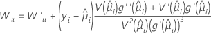
where
This variance-covariance matrix is based on the observed Hessian matrix as opposed to the Fisher's information matrix. Minitab uses the observed Hessian matrix because the model that results is more robust against any conditional mean misspecification.
If the canonical link is used then the observed Hessian matrix and the Fisher's information matrix are identical.
Notation
| Term | Description |
|---|---|
| yi | the response value for the ith row |
 | the estimated mean response for the ith row |
| V(·) | the variance function given in the table below |
| g(·) | the link function |
| V '(·) | the first derivative of the variance function |
| g'(·) | the first derivative of the link function |
| g''(·) | the second derivative of the link function |

See [1] and [2] for more information.
[1] A. Agresti (1990). Categorical Data Analysis. John Wiley & Sons, Inc.
[2] P. McCullagh and J.A. Nelder (1992). Generalized Linear Model. Chapman & Hall.