In This Topic
- Step 1: Determine which terms have the greatest effect on the response
- Step 2: Determine which terms have statistically significant effects on the response
- Step 3: Understand the effects of the predictors
- Step 4: Determine how well the model fits your data
- Step 5: Determine whether the model does not fit the data
Step 1: Determine which terms have the greatest effect on the response
Use a Pareto chart of the standardized effects to compare the relative magnitude and the statistical significance of main, square, and interaction effects.
Minitab plots the standardized effects in the decreasing order of their absolute values. The reference line on the chart indicates which effects are significant. By default, Minitab uses a significance level of 0.05 to draw the reference line.
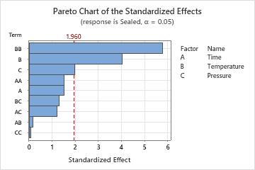
Key Results: Pareto Chart
In these results, the squared term for Temperature (BB) and the main effects for Temperature (B) and Pressure (C) are significant at the α = 0.05 significance level.
In addition, you can see that the largest effect is Temperature*Temperature (BB) because it extends the farthest. Pressure*Pressure (CC) is the smallest because it extends the least.
Step 2: Determine which terms have statistically significant effects on the response
To determine whether the association between the response and each term in the model is statistically significant, compare the p-value for the term to your significance level to assess the null hypothesis. The null hypothesis is that the term's coefficient is equal to zero, which implies that there is no association between the term and the response. Usually, a significance level (denoted as α or alpha) of 0.05 works well. A significance level of 0.05 indicates a 5% risk of concluding that an association exists when there is no actual association.
- P-value ≤ α: The association is statistically significant
- If the p-value is less than or equal to the significance level, you can conclude that there is a statistically significant association between the response variable and the term.
- P-value > α: The association is not statistically significant
- If the p-value is greater than the significance level, you cannot conclude that there is a statistically significant association between the response variable and the term. You may want to refit the model without the term.
- If a coefficient for a factor is significant, you can conclude that the probability of the event is not the same for all levels of the factor.
- If a coefficient for a squared term is significant, you can conclude that the relationship between the factor and the response follows a curved line.
- If a coefficient for an interaction term is significant, the relationship between a factor and the response depends on the other factors in the term. In this case, you should not interpret the main effects without considering the interaction effect.
- If the coefficient for a block is statistically significant, you can conclude that the link function for the block is different from the average value.
Coded Coefficients
| Term | Coef | SE Coef | VIF |
|---|---|---|---|
| Constant | 3.021 | 0.384 | |
| Time | 0.210 | 0.139 | 18.53 |
| Temperature | 0.641 | 0.159 | 19.53 |
| Pressure | 0.420 | 0.211 | 70.48 |
| Time*Time | -0.0735 | 0.0482 | 1.01 |
| Temperature*Temperature | 0.2988 | 0.0517 | 1.17 |
| Pressure*Pressure | -0.0022 | 0.0277 | 70.24 |
| Time*Temperature | -0.0092 | 0.0505 | 1.14 |
| Time*Pressure | 0.0417 | 0.0342 | 18.12 |
| Temperature*Pressure | -0.0521 | 0.0396 | 19.24 |
Key Results: Coefficients
In these results, the coefficients for the main effects of Time, Temperature, and Pressure are positive numbers. The coefficient for the squared term of Time*Time is a negative number. Generally, positive coefficients make the event more likely and negative coefficients make the event less likely as the value of the term increases.
Analysis of Variance
| Source | DF | Adj Dev | Adj Mean | Chi-Square | P-Value |
|---|---|---|---|---|---|
| Model | 9 | 903.478 | 100.386 | 903.48 | 0.000 |
| Time | 1 | 2.303 | 2.303 | 2.30 | 0.129 |
| Temperature | 1 | 16.388 | 16.388 | 16.39 | 0.000 |
| Pressure | 1 | 3.966 | 3.966 | 3.97 | 0.046 |
| Time*Time | 1 | 2.331 | 2.331 | 2.33 | 0.127 |
| Temperature*Temperature | 1 | 34.012 | 34.012 | 34.01 | 0.000 |
| Pressure*Pressure | 1 | 0.006 | 0.006 | 0.01 | 0.937 |
| Time*Temperature | 1 | 0.033 | 0.033 | 0.03 | 0.856 |
| Time*Pressure | 1 | 1.490 | 1.490 | 1.49 | 0.222 |
| Temperature*Pressure | 1 | 1.731 | 1.731 | 1.73 | 0.188 |
| Error | 5 | 23.404 | 4.681 | ||
| Total | 14 | 926.882 |
Key Results: P-Value
In these results, the squared term for Temperature*Temperature and the main effects for Temperature and Pressure are significant at the α = 0.05 significance level.
Step 3: Understand the effects of the predictors
- Odds Ratios for Continuous Predictors
-
Odds ratios that are greater than 1 indicate that the event is more likely to occur as the predictor increases. Odds ratios that are less than 1 indicate that the event is less likely to occur as the predictor increases.
Odds Ratios for Continuous Predictors
Unit of
ChangeOdds Ratio 95% CI Dose (mg) 0.5 6.1279 (1.7218, 21.8087) Key Result: Odds Ratio
In these results, the model uses the dosage level of a medicine to predict the presence or absence of bacteria in adults. In this example, the absence of bacteria is the Event. Each pill contains a 0.5 mg dose, so the researchers use a unit change of 0.5 mg. The odds ratio is approximately 6. For each additional pill that an adult takes, the odds that a patient does not have the bacteria increase by about 6 times.
- Odds Ratios for Categorical Predictors
-
For categorical predictors, the odds ratio compares the odds of the event occurring at 2 different levels of the predictor. Minitab sets up the comparison by listing the levels in 2 columns, Level A and Level B. Level B is the reference level for the factor. Odds ratios that are greater than 1 indicate that the event is more likely at level A. Odds ratios that are less than 1 indicate that the event is less likely at level A. For information on coding categorical predictors, go to Coding schemes for categorical predictors.
Odds Ratios for Categorical Predictors
Level A Level B Odds Ratio 95% CI Month 2 1 1.1250 (0.0600, 21.0834) 3 1 3.3750 (0.2897, 39.3165) 4 1 7.7143 (0.7461, 79.7592) 5 1 2.2500 (0.1107, 45.7172) 6 1 6.0000 (0.5322, 67.6397) 3 2 3.0000 (0.2547, 35.3325) 4 2 6.8571 (0.6556, 71.7169) 5 2 2.0000 (0.0976, 41.0019) 6 2 5.3333 (0.4679, 60.7946) 4 3 2.2857 (0.4103, 12.7323) 5 3 0.6667 (0.0514, 8.6389) 6 3 1.7778 (0.2842, 11.1200) 5 4 0.2917 (0.0252, 3.3719) 6 4 0.7778 (0.1464, 4.1326) 6 5 2.6667 (0.2124, 33.4861) Key Result: Odds Ratio
In these results, the categorical predictor is the month from the start of a hotel's busy season. The response is whether or not a guest cancels a reservation. In this example, a cancellation is the Event. The largest odds ratio is approximately 7.71, when level A is month 4 and level B is month 1. This indicates that the odds that a guest cancels a reservation in month 4 is approximately 8 times higher than the odds that a guest cancels a reservation in month 1.
Step 4: Determine how well the model fits your data
Note
Many of the model summary and goodness-of-fit statistics are affected by how the data are arranged in the worksheet and whether there is one trial per row or multiple trials per row. The Hosmer-Lemeshow test is unaffected by how the data are arranged and is comparable between one trial per row and multiple trials per row. For more information, go to How data formats affect goodness-of-fit in binary logistic regression.
- Deviance R-sq
-
The higher the deviance R2, the better the model fits your data. Deviance R2 is always between 0% and 100%.
Deviance R2 always increases when you add additional terms to a model. For example, the best 5-term model will always have an R2 that is at least as high as the best 4-term model. Therefore, deviance R2 is most useful when you compare models of the same size.
The data arrangement affects the deviance R2 value. The deviance R2 is usually higher for data with multiple trials per row than for data with a single trial per row. Deviance R2 values are comparable only between models that use the same data format.
Goodness-of-fit statistics are just one measure of how well the model fits the data. Even when a model has a desirable value, you should check the residual plots and goodness-of-fit tests to assess how well a model fits the data.
- Deviance R-sq (adj)
-
Use adjusted deviance R2 to compare models that have different numbers of terms. Deviance R2 always increases when you add a term to the model. The adjusted deviance R2 value incorporates the number of terms in the model to help you choose the correct model.
- AIC, AICc, and BIC
-
Use AIC, AICc, and BIC to compare different models. For each statistic, smaller values are desirable. However, the model with the smallest value for a set of predictors does not necessarily fit the data well. Also use goodness-of-fit tests and residual plots to assess how well a model fits the data.
Model Summary
| Deviance R-Sq | Deviance R-Sq(adj) | AIC | AICc | BIC |
|---|---|---|---|---|
| 97.95% | 76.75% | 105.98 | 171.98 | 114.48 |
Key Results: Deviance R-Sq, Deviance R-Sq (adj), AIC
In these results, the model explains 97.95% of the total deviance in the response variable. For these data, the Deviance R2 value indicates the model provides a good fit to the data. If additional models are fit with different predictors, use the adjusted Deviance R2 value, the AIC value, the AICc value, and the BIC value to compare how well the models fit the data.
Step 5: Determine whether the model does not fit the data
- Incorrect link function
- Omitted higher-order term for variables in the model
- Omitted predictor that is not in the model
- Overdispersion
If the deviation is statistically significant, you can try a different link function or change the terms in the model.
- Deviance: The p-value for the deviance test tends to be lower for data that are have a single trial per row arrangement compared to data that have multiple trials per row, and generally decreases as the number of trials per row decreases. For data with single trials per row, the Hosmer-Lemeshow results are more trustworthy.
- Pearson: The approximation to the chi-square distribution that the Pearson test uses is inaccurate when the expected number of events per row in the data is small. Thus, the Pearson goodness-of-fit test is inaccurate when the data are in the single trial per row format.
- Hosmer-Lemeshow: The Hosmer-Lemeshow test does not depend on the number of trials per row in the data as the other goodness-of-fit tests do. When the data have few trials per row, the Hosmer-Lemeshow test is a more trustworthy indicator of how well the model fits the data.
Response Information
| Variable | Value | Count | Event Name |
|---|---|---|---|
| Spoilage | Event | 506 | Event |
| Non-event | 7482 | ||
| Containers | Total | 7988 |
Goodness-of-Fit Tests
| Test | DF | Chi-Square | P-Value |
|---|---|---|---|
| Deviance | 5 | 0.97 | 0.965 |
| Pearson | 5 | 0.97 | 0.965 |
| Hosmer-Lemeshow | 6 | 0.10 | 1.000 |
Key Results for Event/Trial Format: Response Information, Deviance Test, Pearson Test, Hosmer-Lemeshow Test
In these results, alll of the goodness-of-fit tests have p-values higher than the usual significance level of 0.05. The tests do not provide evidence that the predicted probabilities deviate from the observed probabilities in a way that the binomial distribution does not predict.