In This Topic
- R-sq (adj)
- Variance components
- Expected mean squares
- F-statistic for models with random factors
- How the F-statistics in the ANOVA output are calculated
- Why does my ANOVA output include an "x" beside a p-value in the ANOVA table and the label "Not an exact F-test"?
- About the "Denominator of F-test is zero or undefined" message
- Fitted value
- Residual (Resid)
Balanced ANOVA model
The balanced ANOVA model for three or more factors is a straightforward extension of a two-way analysis of variance model.
A three-factor balanced ANOVA model with factors A, B, and C is:
yijkm = μ + α i+ β j + γ k + (αβ)ij+ (αγ)ik+ (βγ)jk+ (αβγ)ijk+εijkm
If the factors are fixed, Σαi = 0, Σβj = 0, Σγk = 0, Σ(αβ)ij = 0, Σ(αγ)ik = 0, Σ(βγ)jk = 0, Σ(αβγ)ijk = 0 and εijkm are independent N(0, σ2).
If the factors are random, α i, β j , γk, (αβ)ij, (αγ)ik, (βγ)jk, (αβγ)ijk,and εijkmare independent random variables. The variables are normally distributed with mean zero and variances given by V(αi) = σ2α,V(β j) = σ2β,V(γk) = σ2γ, V[(αβ)ij] = σ2αβ, V[(αγ)jk] = σ2αγ, V[(βγ)jk] = σ2βγ, V(εijkm) = σ2.
The three-factor model can be extended to models with more than three factors.
Factor means
Formula
The average of the observations for a factor at a given level. The formulas are:
Mean of Factor A: 
Mean of Factor B: 
Mean of Factor C: 
Overall mean: 
Notation
| Term | Description |
|---|---|
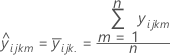
| yi... | sum of all observations for the ith factor level of A |
| y.j.. | sum of all observations for the jth factor level of B |
| y..k. | sum of all observations for the kth factor level of C |
| y.... | sum of all observations in the sample |
| a | number of levels in A |
| b | number of levels in B |
| c | number of levels in C |
| n | number of observations in each combination of the factor and levels |
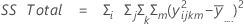
Sum of squares (SS)
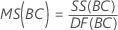
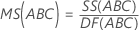
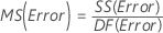
The sum of squared distances. SS Total is the total variation in the data. SS (A), SS (B), and SS (C) represent the amount of variation of estimated factor level mean around the overall mean. They are also known as the sum of squares between treatments. SS(AB), SS(AC), SS(BC) and SS(ABC) represent the amount of variation explained by each respective interaction term. SS Error represents the amount of variation between the fitted value and the actual observation. It is also known as error within treatments. These formulas assume a full model is fit. The calculations are:
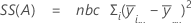
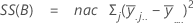
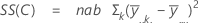


- SS Error = SS Total - SS (for all terms in model)
Notation
| Term | Description |
|---|---|
| a | number of levels in factor A |
| b | number of levels in factor B |
| c | number of levels in factor C |
| n | total number of trials |
 | mean of the ith factor level of factor A |
 | overall mean of all observations |
 | mean of the jth factor level of factor B |
 | mean of the kth factor level of factor C |
 | estimated treatment mean |
Degrees of Freedom (DF)
The degrees of freedom for each component of the model are:
| Sources of variation | DF |
|---|---|
| Factor | ki – 1 |
| Covariates and interactions between covariates | 1 |
| Interactions that involve factors |  |
| Regression | p |
| Error | n – p – 1 |
| Total | n – 1 |
Notation
| Term | Description |
|---|---|
| ki | number of levels in the ith factor |
| m | number of factors |
| n | number of observations |
| p | number of coefficients in the model, not counting the constant |
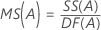
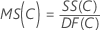
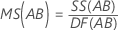
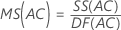
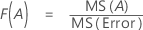
Mean square (MS)
Formulas

F
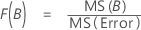
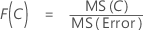
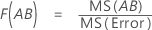
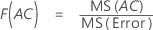
For a 3-factor ANOVA with all fixed factors, these formulas are the F-statistics when the model is full.
Formulas
- For F(A), the degrees of freedom for the numerator are a - 1 and for the denominator are (n - 1)abc.
- For F(B), the degrees of freedom for the numerator are b - 1 and for the denominator are (n - 1)abc.
- For F(C), the degrees of freedom for the numerator are c - 1 and for the denominator are (n - 1)abc.
- For F(AB), the degrees of freedom for the numerator are (a - 1)(b - 1) and for the denominator are (n - 1)abc.
- For F(AC), the degrees of freedom for the numerator are (a - 1)(c - 1) and for the denominator are (n - 1)abc.
- For F(BC), the degrees of freedom for the numerator are (b - 1)(c - 1) and for the denominator are (n - 1)abc.
- For F(ABC), the degrees of freedom for the numerator are (a - 1)(b - 1)(c - 1) and for the denominator are (n - 1)abc.
If there are random factors in the model, the F ratio for each term is determine by the expected mean square for each term.
Larger values of F support rejecting the null hypothesis. You can conclude that the effect is statistically significant.
P-value – Analysis of variance table
The p-value is a probability that is calculated from an F-distribution with the degrees of freedom (DF) as follows:
- Numerator DF
- sum of the degrees of freedom for the term or the terms in the test
- Denominator DF
- degrees of freedom for error
Formula
1 − P(F ≤ fj)
Notation
| Term | Description |
|---|---|
| P(F ≤ f) | cumulative distribution function for the F-distribution |
| f | f-statistic for the test |
S

Notation
| Term | Description |
|---|---|
| MSE | mean square error |
R-sq
R2 is also known as the coefficient of determination.
Formula
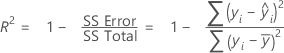
Notation
| Term | Description |
|---|---|
| yi | i th observed response value |
 | mean response |
 | i th fitted response |
R-sq (adj)
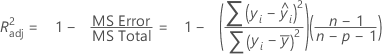
While the calculations for adjusted R2 can produce negative values, Minitab displays zero for these cases.
Notation
| Term | Description |
|---|---|
 | ith observed response value |
 | ith fitted response |
 | mean response |
| n | number of observations |
| p | number of terms in the model |
Variance components

where, αi, βj , (αβ)ij, and εijk are independent random variables. The variables are normally distributed with mean zero and variances given by these formulas:


These variances are the variance components. In this case, test the hypothesis that the variance components are equal to zero.
For a restricted mixed model with two factors, the model is:

where αi is a fixed effect and βj is a random effect, (αβ)ij, is a random effect, and εijk is random error. The Σαi = 0 and Σ(αβ)ij = 0 for each j. The variances are V(βj) = σ2β,V[(αβ)ij] =[(a - 1)/a]σ2αβ, and V(εijk) = σ2. σ2β, σ2αβ, and σ2 are variance components. Summing the interaction component over the fixed factor equals zero, which indicates this is the restricted mixed model.
For an unrestricted mixed model with a fixed factor, A, and a random factor, B, this formula describes the model:

where αi are fixed effects and βj, (αβ)ij and εijk are uncorrelated random variables having zero means and these variances:


These variances are the variance components. The Σα i = 0 and Σ(αβ)ij = 0 for each j.
This information is for balanced models. For information on unbalanced or more complex models, see Montgomery1 and Neter2.
- D.C. Montgomery (1991). Design and Analysis of Experiments, Third Edition. John Wiley & Sons.
- J. Neter, W. Wasserman and M.H. Kutner (1985). Applied Linear Statistical Models, Second Edition. Irwin, Inc.
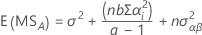
Expected mean squares
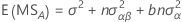


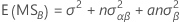
The formulas for the expected mean squares for a restricted mixed model with two factors, A (fixed) and B (random) are:
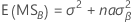


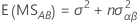
The formulas for the expected mean squares for an unrestricted mixed model with a fixed factor, A, and a random factor, B, are:
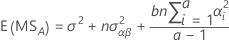

For the general rules on calculating expected mean squares, and for information on unbalanced or more complex models, see Montgomery1 and Neter2.
- D.C. Montgomery (1991). Design and Analysis of Experiments, Third Edition. John Wiley & Sons.
- J. Neter, W. Wasserman and M.H. Kutner (1985). Applied Linear Statistical Models, Second Edition. Irwin, Inc.
Notation
| Term | Description |
|---|---|
| b | number of levels in factor B |
| a | number of levels in factor A |
| n | number of observations |
| σ2 | estimated variance of the model |
 | estimated variance of A |
 | estimated variance of B |
 | estimated variance of AB |
 | fixed effects of A |
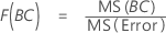
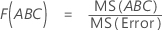
F-statistic for models with random factors
How the F-statistics in the ANOVA output are calculated
Each F-statistic is a ratio of mean squares. The numerator is the mean square for the term. The denominator is chosen such that the expected value of the numerator mean square differs from the expected value of the denominator mean square only by the effect of interest. The effect for a random term is represented by the variance component of the term. The effect for a fixed term is represented by the sum of squares of the model components associated with that term divided by its degrees of freedom. Therefore, a high F-statistic indicates a significant effect.
When all the terms in the model are fixed, the denominator for each F-statistic is the mean square of the error (MSE). However, for models that include random terms, the MSE is not always the correct mean square. The expected mean squares (EMS) can be used to determine which is appropriate for the denominator.
Example
| Source | Expected Mean Square for Each Term |
|---|---|
| (1) Screen | (4) + 2.0000(3) + Q[1] |
| (2) Tech | (4) + 2.0000(3) + 4.0000(2) |
| (3) Screen*Tech | (4) + 2.0000(3) |
| (4) Error | (4) |
A number with parentheses indicates a random effect associated with the term listed beside the source number. (2) represents the random effect of Tech, (3) represents the random effect of the Screen*Tech interaction, and (4) represents the random effect of Error. The EMS for Error is the effect of the error term. In addition, the EMS for Screen*Tech is the effect of the error term plus two times the effect of the Screen*Tech interaction.
To calculate the F-statistic for Screen*Tech, the mean square for Screen*Tech is divided by the mean square of the error so that the expected value of the numerator (EMS for Screen*Tech = (4) + 2.0000(3)) differs from the expected value of the denominator (EMS for Error = (4)) only by the effect of the interaction (2.0000(3)). Therefore, a high F-statistic indicates a significant Screen*Tech interaction.
A number with Q[ ] indicates the fixed effect associated with the term listed beside the source number. For example, Q[1] is the fixed effect of Screen. The EMS for Screen is the effect of the error term plus two times the effect of the Screen*Tech interaction plus a constant times the effect of Screen. Q[1] equals (b*n * sum((coefficients for levels of Screen)**2)) divided by (a - 1), where a and b are the number of levels of Screen and Tech, respectively, and n is the number of replicates.
To calculate the F-statistic for Screen, the mean square for Screen is divided by the mean square for Screen*Tech so that the expected value of the numerator (EMS for Screen = (4) + 2.0000(3) + Q[1] ) differs from the expected value of the denominator (EMS for Screen*Tech = (4) + 2.0000(3) ) only by the effect due to the Screen (Q[1]). Therefore, a high F-statistic indicates a significant Screen effect.
Why does my ANOVA output include an "x" beside a p-value in the ANOVA table and the label "Not an exact F-test"?
An exact F-test for a term is one in which the expected value of the numerator mean squares differs from the expected value of the denominator mean squares only by the variance component or the fixed factor of interest.
Sometimes, however, such a mean square cannot be calculated. In this case, Minitab uses a mean square that results in an approximate F-test and displays an "x" beside the p-value to identify that the F-test is not exact.
| Source | Expected Mean Square for Each Term |
|---|---|
| (1) Supplement | (4) + 1.7500(3) + Q[1] |
| (2) Lake | (4) + 1.7143(3) + 5.1429(2) |
| (3) Supplement*Lake | (4) + 1.7500(3) |
| (4) Error | (4) |
The F-statistic for Supplement is the mean square for Supplement divided by the mean square for the Supplement*Lake interaction. If the effect for Supplement is very small, the expected value of the numerator equals the expected value of the denominator. This is an example of an exact F-test.
Notice, however, that for a very small Lake effect, there are no mean squares such that the expected value of the numerator equals the expected value of the denominator. Therefore, Minitab uses an approximate F-test. In this example, the mean square for Lake is divided by the mean square for the Supplement*Lake interaction. This results in an expected value of the numerator being approximately equal to that of the denominator if the Lake effect is very small.
About the "Denominator of F-test is zero or undefined" message
- There is not at least one degree of freedom for error.
-
The adjusted MS values are very small, and thus there is not enough precision to display the F and p-values. As a workaround, multiply the response column by 10. Then perform the same regression model, but instead use this new response column for the response.
Note
Multiplying the response values by 10 will not affect the F and p-values that Minitab displays the output. However, decimal position will be affected in the remaining output, specifically, the sequential sums of squares, Adj SS, Adj MS, Fit, standard error of the fits, and residual columns.
Fitted value
Notation
For a 3-factor model:
| Term | Description |
|---|---|
 | the fitted value for the observation at the ith level of factor A, the jth level of factor B, the kth level of factor C |
 | the mean value for the observation at the ith level of factor A, the jth level of factor B, the kth level of factor C |
| n | the number of observations at the ith level of factor A, the jth level of factor B, the kth level of factor C |
Residual (Resid)

Notation
| Term | Description |
|---|---|
| ei | i th residual |
 | i th observed response value |
 | i th fitted response |