In This Topic
Parameter
The parameter shows the statistic that you selected in the dialog. Parameters are descriptive measures of an entire population used as the inputs for a probability distribution function (PDF) to generate distribution curves. For more information, go to What are parameters, parameter estimates, and sampling distributions?
Length of observation
Poisson processes count occurrences of a certain event or property on a specific observation range, which can represent things such as time, area, volume, and number of items. The length of observation represents the magnitude, duration, or size of each observation range.
Interpretation
Minitab uses the length of observation to convert the rate of occurrence into a form that is best for your situation.
For example, if each sample observation counts the number of events in a year, a length of 1 represents a yearly rate of occurrence, and a length of 12 represents a monthly rate of occurrence.
- The total occurrences is 122 because the inspectors find 122 defects.
- The sample size (N) is 50 because the inspectors sample 50 boxes.
- To determine the number of defects per towel, inspectors use a length of observation of 10 because each box contains 10 towels. To determine the number of defects per box, inspectors use a length of observation of 1.
- The rate of occurrence is (Total occurrences / N) / (length of observation) = (122/50) / 10 = 0.244. So, on average, each towel has 0.244 defects.
Distribution
- Normal
-
The normal distribution is a bell-shaped distribution in which successive standard deviations from the mean establish benchmarks for estimating the percentage of data observations. These benchmarks are the basis behind many hypothesis tests such as Z- and t-tests.
For example, the heights of all adult males who live in the state of Pennsylvania are approximately normally distributed. Therefore, the heights of most men are close to the mean height of 69 inches. A similar number of men are slightly taller and slightly shorter than 69 inches. Only a few are much taller or much shorter.
- Binomial
-
When you independently classify items, event, or people into one of two categories, then the number of items, events, or people in one category follows the binomial distribution. The two categories should be mutually exclusive, such as yes/no, pass/fail, or defective/nondefective.
For example, engineers examine a sample of bolts for severe cracks that make the bolts unusable. Bolts that do not have a crack are nondefective, and bolts that have a crack are defective.
- Poisson
-
When you count the presence of a characteristic, result, or activity over a certain amount of time, area, or other length of observation, you obtain Poisson data. Poisson data are evaluated in counts per unit, with the units the same size.
For example, inspectors at a bus company count the number of bus breakdowns each day for 30 days.
Standard deviation
The standard deviation is the most common measure of dispersion, or how spread out the data are about the mean. The symbol σ (sigma) is often used to represent the standard deviation of a population, while s is used to represent the standard deviation of a sample. Variation that is random or natural to a process is often referred to as noise. The value Minitab displays is the planning value you specified in the dialog.
Proportion
A proportion is a relative portion of a whole, as opposed to a count or frequency. The proportion equals the number of events divided by the sample size. The value Minitab displays is the planning value you specified in the dialog.
Rate
The rate of occurrence of an event is the average number of times the event occurs per unit length of observation. The value Minitab displays is the planning value you specified in the dialog.
Mean
A Poisson mean is the average number of times an event occurs across the total observation space. The value Minitab displays is the planning value you specified in the dialog.
Confidence level
A confidence level of 95% usually works well. This indicates that 19 out of 20 samples (95%) from the same population will produce confidence intervals that contain the population parameter.
The confidence level represents the percentage of intervals that would include the population parameter if you took samples from the same population again and again. Thus, if you collected 100 samples, and made 100 95% confidence intervals, you would expect approximately 95 of the intervals to contain the population parameter, such as the mean of the population, as shown in the following figure.
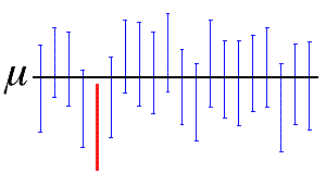
In the figure, the horizontal line represents the fixed value of the unknown population mean, µ. The 19 vertical blue confidence intervals that overlap the horizontal line contain the value of the population mean. The 1 red confidence interval that is completely below the horizontal line does not.
Confidence interval
Minitab displays the type of confidence interval you specified in the dialog.
The confidence interval provides a range of likely values for the population proportion. Because samples are random, two samples from a population are unlikely to yield identical confidence intervals. But, if you repeated your sample many times, a certain percentage of the resulting confidence intervals or bounds would contain the unknown population parameter. The percentage of these confidence intervals or bounds that contain the parameter is the confidence level of the interval.
An upper bound defines a value that the population parameter is likely to be less than. A lower bound defines a value that the population parameter is likely to be greater than.