In This Topic
Mean
The Poisson mean is the sum of each category multiplied by the number of values observed in that category divided by the total number of observed values.
N
The number of non-missing values in the sample.
| Total count | N | N* |
|---|---|---|
| 149 | 141 | 8 |
N*
The number of missing values in the sample. The number of missing values refers to cells that contain the missing value symbol *.
| Total count | N | N* |
|---|---|---|
| 149 | 141 | 8 |
Poisson Probability
The probability for each category, assuming that the data follow a Poisson distribution that has a mean that is equal to the Poisson mean that is calculated from the data. Minitab uses the Poisson probability to calculate the expected values.
Observed and expected values
The observed values are the actual number of observations in a sample that belong to a category.
The expected values are the number of observations that would be expected if the Poisson probabilities were true. Minitab calculates the expected counts by multiplying the Poisson probabilities from each category by the total sample size.
If the expected counts (also called expected frequencies) for any category is less than 5, the results of the test may not be valid. If the expected counts for a category are too low, you may be able to combine that category with adjacent categories to achieve the minimum expected count.
For example, a finance department has five categories to classify the number of days that invoices are overdue: 15 or less, 16–30, 31–45, 46–60, and 60 or more. The category for 60 days or more has a low expected count, so the finance department combines it with the category for 46–60 days to create a combined category for 45 days or more.
Interpretation
You can compare the observed values and the expected values by using the output table or the bar chart. Larger differences between observed and expected values indicate that the data do not follow a Poisson distribution.
Method
| Frequencies in Observed |
|---|
Descriptive Statistics
| N | Mean |
|---|---|
| 300 | 0.536667 |
Observed and Expected Counts for Defects
| Defects | Poisson Probability | Observed Count | Expected Count | Contribution to Chi-Square |
|---|---|---|---|---|
| 0 | 0.584694 | 213 | 175.408 | 8.056 |
| 1 | 0.313786 | 41 | 94.136 | 29.993 |
| 2 | 0.084199 | 18 | 25.260 | 2.086 |
| >=3 | 0.017321 | 28 | 5.196 | 100.072 |
Chi-Square Test
| Null hypothesis | H₀: Data follow a Poisson distribution |
|---|---|
| Alternative hypothesis | H₁: Data do not follow a Poisson distribution |
| DF | Chi-Square | P-Value |
|---|---|---|
| 2 | 140.208 | 0.000 |
Contribution to Chi-Sq
Use the individual category contributions to quantify how much of the total chi-square statistic is attributable to each category's divergence.
Minitab calculates each category's contribution to the chi-square statistic as the square of the difference between the observed and expected values for a category, divided by the expected value for that category. The chi-square statistic is the sum of these values for all categories.
Interpretation
Categories with a large difference between observed and expected values make a larger contribution to the overall chi-square statistic.
In these results, the chi-square values from each category sum to the overall chi-square statistic, which is 140.208. The largest contribution comes from the 3 or more defects category. This result indicates that the largest difference between observed and expected counts is in the 3 or more defects category. The smallest difference between observed and expected counts is in the 2 defects category.
Method
| Frequencies in Observed |
|---|
Descriptive Statistics
| N | Mean |
|---|---|
| 300 | 0.536667 |
Observed and Expected Counts for Defects
| Defects | Poisson Probability | Observed Count | Expected Count | Contribution to Chi-Square |
|---|---|---|---|---|
| 0 | 0.584694 | 213 | 175.408 | 8.056 |
| 1 | 0.313786 | 41 | 94.136 | 29.993 |
| 2 | 0.084199 | 18 | 25.260 | 2.086 |
| >=3 | 0.017321 | 28 | 5.196 | 100.072 |
Chi-Square Test
| Null hypothesis | H₀: Data follow a Poisson distribution |
|---|---|
| Alternative hypothesis | H₁: Data do not follow a Poisson distribution |
| DF | Chi-Square | P-Value |
|---|---|---|
| 2 | 140.208 | 0.000 |
Null and alternative hypotheses
- Null hypothesis
- The null hypothesis states that a population follows a specific distribution. The null hypothesis is often an initial claim that is based on previous analyses or specialized knowledge.
- Alternative hypothesis
- The alternative hypothesis states that a population does not follow a specific distribution.
DF
Degrees of freedom (DF) is the number of independent pieces of information about a statistic. The degrees of freedom for the goodness-of-fit test for Poisson is the number of categories – 2.
Interpretation
Minitab uses the degrees of freedom to determine the test statistic. The more categories you have in your study, the more degrees of freedom you have.
Chi-Square
The chi-square statistic is a test statistic that measures the amount of divergence between the distribution of your sample data and an expected Poisson distribution.
Interpretation
You can use the chi-square statistic to determine whether to reject the null hypothesis. However, the p-value is used more often because it is easier to interpret. The p-value is the probability of obtaining a test statistic (such as the chi-square statistic) that is at least as extreme as the value that is calculated from the sample, when the data follow a Poisson distribution.
To determine whether to reject the null hypothesis, compare the chi-square statistic to your critical value. If the chi-square statistic is greater than the critical value, you reject the null hypothesis. If it is not, you fail to reject the null hypothesis. You can calculate the critical value in Minitab or find the critical value from a chi-square distribution table in most statistics books. For more information, go to Using the inverse cumulative distribution function (ICDF) and click "Use the ICDF to calculate critical values".
Minitab uses the chi-square statistic to calculate the p-value.
P-Value
The p-value is a probability that measures the evidence against the null hypothesis. A smaller p-value provides stronger evidence against the null hypothesis.
Interpretation
Use the p-value to determine whether the data do not follow a Poisson distribution.
- P-value ≤ α: The data do not follow a Poisson distribution (Reject H0)
- If the p-value is less than or equal to the significance level, the decision is to reject the null hypothesis and conclude that your data do not follow a Poisson distribution.
- P-value > α: You cannot conclude that the data do not follow a Poisson distribution (Fail to reject H0)
- If the p-value is larger than the significance level, the decision is to fail to reject the null hypothesis because you do not have enough evidence to conclude that your data do not follow a Poisson distribution.
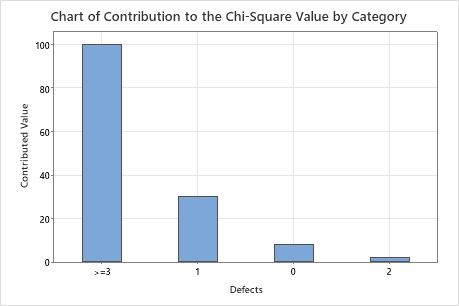
Chart of Contribution to the Chi-Square Value by Category
This bar chart plots each category's contribution to the overall chi-square statistic. You can choose a chart that orders the categories by contribution, from largest contribution to smallest contribution.
Interpretation
Categories with a large difference between observed and expected values make a larger contribution to the overall chi-square statistic.
This bar chart indicates that the largest difference between the expected and observed values is in the 3 or more defects category.
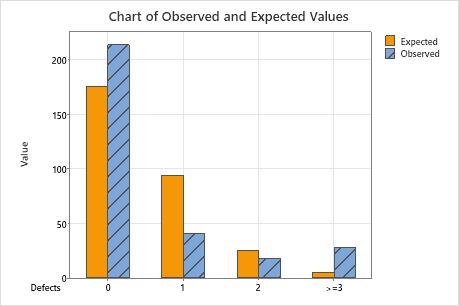
Chart of Observed and Expected Values
Use a bar chart of observed and expected values to determine whether, for each category, the number of observed values differs from the number of expected values. Larger differences between observed and expected values indicate that the data do not follow a Poisson distribution.
This bar chart indicates that the observed values for 0 defects, 1 defect, and more than 3 defects are different from the expected values. Thus, the bar chart visually confirms what the p-value indicates, which is that the data do not follow a Poisson distribution.