A classification tree results from a binary recursive partitioning of the original training data set. Any parent node (a subset of training data) in a tree can be split into two mutually exclusive child nodes in a finite number of ways, which depends on the actual data values collected in the node.
The splitting procedure treats predictor variables as either continuous or categorical. For a continuous variable X and a value c, a split is defined by sending all records with the values of X less than or equal than c to the left node, and all remaining records to the right node. CART always uses the average of two adjacent values to compute c. A continuous variable with N distinct values generates up to N–1 potential splits of the parent node (the actual number will be smaller when limits on the minimum allowed node size are imposed).
For example, a continuous predictor has the values 55, 66, and 75 in the data. One possible split for this variable is to send all values less than or equal to (55+66)/2 = 60.5 to one child node and all values greater than 60.5 to the other child node. Cases with the predictor value of 55 go to one node and the cases with the values 66 and 75 go to the other node. The other possible split for this predictor is to send all values less than or equal to 70.5 to one child node and values greater than 70.5 to the other node. Cases with the values 55 and 66 go to one node, and cases with the value 75 go to the other node.
For a categorical variable X with distinct values {c1, c2, …, ck}, a split is defined as a subset of levels that are sent to the left child node. A categorical variable with K levels generates up to 2K-1–1 splits.
| Left Child Node | Right Child Node |
|---|---|
| Red, Blue | Yellow |
| Red, Yellow | Blue |
| Blue, Yellow | Red |
In classification trees, the target is multinomial with K distinct classes. The main goal of the tree is to find a way to separate different target classes into individual nodes in as pure way as possible. The resulting number of terminal nodes do not need to be K; multiple terminal nodes can be used to represent a specific target class. A user can specify prior probabilities for the target classes; these will be accounted by CART during the tree growing process.
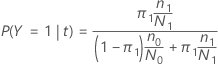
In the following sections, Minitab uses the following definitions for a binary response variable:

In the following sections, Minitab uses the following definitions for a multinomial response variable:
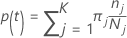
The probability of class j given node t:

These definitions give the within-node probabilities. Minitab calculates these probabilities for any node and any potential split. Minitab calculates the overall improvement for a potential split from these probabilities with one of the following criteria.
Notation
| Term | Description |
|---|---|
| K | number of classes in the response variable |
 | prior probability for class j |
 | number of observations for class j in a node |
 | number of observations for class j in the data |
Gini criterion

The following more general formula applies to a multinomial response variable:
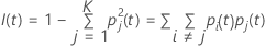
Note that if all of the observations for a node are in one class, then
 .
.
Entropy criterion

The following more general formula applies to a multinomial response variable:
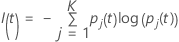
Note that if all of the observations for a node are in one class, then
 .
.
Twoing criterion
| Super Class 1 | Super Class 2 |
|---|---|
| 1, 2, 3 | 4 |
| 1, 2, 3 | 3 |
| 1, 3, 4 | 2 |
| 2, 3, 4 | 1 |
| 1, 2 | 3, 4 |
| 1, 3 | 2, 4 |
| 1, 4 | 2, 3 |


The left super class has all of the target classes that tend to go left. The right super class has all of the target classes that tend to go right.
| Class | Left Child Node Probability | Right Child Node Probability |
|---|---|---|
| 1 | 0.67 | 0.33 |
| 2 | 0.82 | 0.18 |
| 3 | 0.23 | 0.77 |
| 4 | 0.89 | 0.11 |
Then the best way to make the super classes for the candidate split is to assign {1, 2, 4} as one super class and {3} as the other super class.
The rest of the calculation is the same as the for the Gini criterion with the super classes as the binary target.
Improvement calculation for the criteria
After Minitab computes the node impurity, Minitab computes the conditional probabilities for splitting the node with a predictor:

and

Then, the improvement for a split is from the following formula:

The split with the highest improvement value becomes part of the tree. If the improvement for two predictors is the same, the algorithm requires a selection to proceed. The selection uses a deterministic tie-breaking scheme that involves the position of the predictors in the worksheet, the type of predictor, and the number of classes in a categorical predictor.
Class probability
Node splits maximize the probability of a class within a given node.
Terminal nodes
- The number of cases in the node reaches the minimum size for the analysis. The default minimum in Minitab Statistical Software is 3.
- All the cases in a node have the same response class.
- All the cases in a node have the same predictor values.
Predicted class for a terminal node
The predicted class for a terminal node is the class that minimizes the misclassification cost for the node. Representations of the misclassification cost depend on the number of classes in the response variable. Because the predicted class for a terminal node comes from the training data when you use a validation method, all of the following formulas use probabilities from the training data set.
Binary response variable
The following equation gives the misclassification cost for the prediction that the cases in the node are the event class:

The following equation gives the misclassification cost for the prediction that the case in the node are the non-event class:

| Term | Description |
|---|---|
| PY=0|t | conditional probability that a case in node t belongs to the non-event class |
| C1|0 | misclassification cost that a nonevent class case is predicted as an event class case |
| PY=1|t | conditional probability that a case in node t belongs to the event class |
| C0|1 | misclassification cost that an event class case is predicted as a nonevent class case |
The predicted class for a terminal node is the class with the minimum misclassification cost.
Multinomial response variable

For example, consider a response variable with three classes and the following misclassification costs:
| Predicted Class | |||
| Actual class | 1 | 2 | 3 |
| 1 | 0.0 | 4.1 | 3.2 |
| 2 | 5.6 | 0.0 | 1.1 |
| 3 | 0.4 | 0.9 | 0.0 |
Then, consider that the classes of the response variable have the following probabilities for node t:


The least misclassification cost is for the prediction that Y = 3, 1.164. This class is the predicted class for the terminal node.