The supervisor for a call center wants to evaluate the process for answering customer phone calls. The supervisor records the total number of incoming calls and the number of unanswered calls for 21 days.
The supervisor performs binomial capability analysis to evaluate how well the process for answering calls meets specifications.
- Open the sample data, UnansweredCalls.MWX.
- Choose .
- In Defectives, enter Unanswered Calls.
- Under Sample size, select Use sizes in and enter Total Calls.
- Click OK.
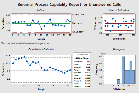
Interpret the results
On the Rate of Defectives plot, the points appear to be randomly distributed across the various sample sizes, so the supervisor can assume that sample size does not affect the rate of defectives. The P chart and the Cumulative %Defective plot indicate that the %defective is fairly stable for this process. Therefore, the assumptions for the capability analysis appear to be satisfied.
In the Summary Stats table, the parts per million defective (PPM Def) indicates that 95,657 calls out 1,000,000 are expected to be unanswered (defective). This PPM value corresponds to a %defective of approximately 9.57%. The upper and lower confidence limits (CI) indicate that the supervisor can be 95% confident that the %defective for the process is contained within the interval 8.79% and 10.39%. The Process Z value of 1.3 is lower than 2, which is often considered the minimum required value for a capability process. Together, these summary statistics indicate that the call center is not capable of meeting specifications. A high percentage of calls are unanswered. The supervisor needs to determine why so many calls are unanswered and how to improve the process.