In This Topic
Step 1: Determine the number of principal components
- Proportion of variance that the components explain
- Use the cumulative proportion to determine the amount of variance that the principal components explain. Retain the principal components that explain an acceptable level of variance. The acceptable level depends on your application. For descriptive purposes, you may only need 80% of the variance explained. However, if you want to perform other analyses on the data, you may want to have at least 90% of the variance explained by the principal components.
- Eigenvalues
- You can use the size of the eigenvalue to determine the number of principal components. Retain the principal components with the largest eigenvalues. For example, using the Kaiser criterion, you use only the principal components with eigenvalues that are greater than 1.
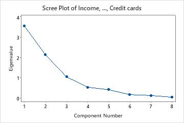
- Scree plot
- The scree plot orders the eigenvalues from largest to smallest. The ideal pattern is a steep curve, followed by a bend, and then a straight line. Use the components in the steep curve before the first point that starts the line trend.
Eigenanalysis of the Correlation Matrix
| Eigenvalue | 3.5476 | 2.1320 | 1.0447 | 0.5315 | 0.4112 | 0.1665 | 0.1254 | 0.0411 |
|---|---|---|---|---|---|---|---|---|
| Proportion | 0.443 | 0.266 | 0.131 | 0.066 | 0.051 | 0.021 | 0.016 | 0.005 |
| Cumulative | 0.443 | 0.710 | 0.841 | 0.907 | 0.958 | 0.979 | 0.995 | 1.000 |
Eigenvectors
| Variable | PC1 | PC2 | PC3 | PC4 | PC5 | PC6 | PC7 | PC8 |
|---|---|---|---|---|---|---|---|---|
| Income | 0.314 | 0.145 | -0.676 | -0.347 | -0.241 | 0.494 | 0.018 | -0.030 |
| Education | 0.237 | 0.444 | -0.401 | 0.240 | 0.622 | -0.357 | 0.103 | 0.057 |
| Age | 0.484 | -0.135 | -0.004 | -0.212 | -0.175 | -0.487 | -0.657 | -0.052 |
| Residence | 0.466 | -0.277 | 0.091 | 0.116 | -0.035 | -0.085 | 0.487 | -0.662 |
| Employ | 0.459 | -0.304 | 0.122 | -0.017 | -0.014 | -0.023 | 0.368 | 0.739 |
| Savings | 0.404 | 0.219 | 0.366 | 0.436 | 0.143 | 0.568 | -0.348 | -0.017 |
| Debt | -0.067 | -0.585 | -0.078 | -0.281 | 0.681 | 0.245 | -0.196 | -0.075 |
| Credit cards | -0.123 | -0.452 | -0.468 | 0.703 | -0.195 | -0.022 | -0.158 | 0.058 |
Key Results: Cumulative, Eigenvalue, Scree Plot
In these results, the first three principal components have eigenvalues greater than 1. These three components explain 84.1% of the variation in the data. The scree plot shows that the eigenvalues start to form a straight line after the third principal component. If 84.1% is an adequate amount of variation explained in the data, then you should use the first three principal components.
Step 2: Interpret each principal component in terms of the original variables
To interpret each principal components, examine the magnitude and direction of the coefficients for the original variables. The larger the absolute value of the coefficient, the more important the corresponding variable is in calculating the component. How large the absolute value of a coefficient has to be in order to deem it important is subjective. Use your specialized knowledge to determine at what level the correlation value is important.
Eigenanalysis of the Correlation Matrix
| Eigenvalue | 3.5476 | 2.1320 | 1.0447 | 0.5315 | 0.4112 | 0.1665 | 0.1254 | 0.0411 |
|---|---|---|---|---|---|---|---|---|
| Proportion | 0.443 | 0.266 | 0.131 | 0.066 | 0.051 | 0.021 | 0.016 | 0.005 |
| Cumulative | 0.443 | 0.710 | 0.841 | 0.907 | 0.958 | 0.979 | 0.995 | 1.000 |
Eigenvectors
| Variable | PC1 | PC2 | PC3 | PC4 | PC5 | PC6 | PC7 | PC8 |
|---|---|---|---|---|---|---|---|---|
| Income | 0.314 | 0.145 | -0.676 | -0.347 | -0.241 | 0.494 | 0.018 | -0.030 |
| Education | 0.237 | 0.444 | -0.401 | 0.240 | 0.622 | -0.357 | 0.103 | 0.057 |
| Age | 0.484 | -0.135 | -0.004 | -0.212 | -0.175 | -0.487 | -0.657 | -0.052 |
| Residence | 0.466 | -0.277 | 0.091 | 0.116 | -0.035 | -0.085 | 0.487 | -0.662 |
| Employ | 0.459 | -0.304 | 0.122 | -0.017 | -0.014 | -0.023 | 0.368 | 0.739 |
| Savings | 0.404 | 0.219 | 0.366 | 0.436 | 0.143 | 0.568 | -0.348 | -0.017 |
| Debt | -0.067 | -0.585 | -0.078 | -0.281 | 0.681 | 0.245 | -0.196 | -0.075 |
| Credit cards | -0.123 | -0.452 | -0.468 | 0.703 | -0.195 | -0.022 | -0.158 | 0.058 |
Key Results: PC, Loading plot
In these results, first principal component has large positive associations with Age, Residence, Employ, and Savings, so this component primarily measures long-term financial stability. The second component has large negative associations with Debt and Credit cards, so this component primarily measures an applicant's credit history. The third component has large negative associations with income, education, and credit cards, so this component primarily measures the applicant's academic and income qualifications.
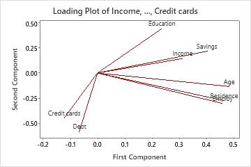
The loading plot visually shows the results for the first two components. Age, Residence, Employ, and Savings have large positive loadings on component 1, so this component measure long-term financial stability. Debt and Credit Cards have large negative loadings on component 2, so this component primarily measures an applicant's credit history.
Step 3: Identify outliers
Use the outlier plot to identify outliers. Any point that is above the reference line is an outlier. Outliers can significantly affect the results of your analysis. Therefore, if you identify an outlier in your data, you should examine the observation to understand why it is unusual. Correct any measurement or data entry errors. Consider removing data that are associated with special causes and repeating the analysis.
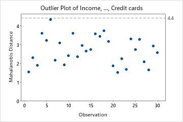
Key Result: Outlier Plot
In these results, there are no outliers. All the points are below the reference line.
Tip
Hold your pointer over any point on an outlier plot to identify the observation. Use to brush multiple outliers on the plot and flag the observations in the worksheet.