In This Topic
- Step 1: Test the equality of means from all the responses
- Step 2: Determine which response means have the largest differences for each factor
- Step 3: Assess the differences between group means
- Step 4: Assess the univariate results to examine individual responses
- Step 5: Determine whether your model meets the assumptions of the analysis
Step 1: Test the equality of means from all the responses
- P-value ≤ α: The differences between the means are statistically significant
- If the p-value is less than or equal to the significance level, you can conclude that the differences between the means are statistically significant.
- P-value > α: The differences between the means are not statistically significant
- If the p-value is greater than the significance level, you cannot conclude that the differences between the means are statistically significant. You may want to refit the model without the term.
- If a main effect is significant, the level means for the factor are significantly different from each other across all responses in your model.
- If an interaction term is significant, the effects of each factor are different at each level of the other factors across all responses in your model. For this reason, you should not analyze the individual effects of terms involved in significant higher-order interactions.
MANOVA Tests for Method
| Test Statistic | DF | ||||
|---|---|---|---|---|---|
| Criterion | F | Num | Denom | P | |
| Wilks' | 0.63099 | 16.082 | 2 | 55 | 0.000 |
| Lawley-Hotelling | 0.58482 | 16.082 | 2 | 55 | 0.000 |
| Pillai's | 0.36901 | 16.082 | 2 | 55 | 0.000 |
| Roy's | 0.58482 | ||||
MANOVA Tests for Plant
| Test Statistic | DF | ||||
|---|---|---|---|---|---|
| Criterion | F | Num | Denom | P | |
| Wilks' | 0.89178 | 1.621 | 4 | 110 | 0.174 |
| Lawley-Hotelling | 0.11972 | 1.616 | 4 | 108 | 0.175 |
| Pillai's | 0.10967 | 1.625 | 4 | 112 | 0.173 |
| Roy's | 0.10400 | ||||
MANOVA Tests for Method*Plant
| Test Statistic | DF | ||||
|---|---|---|---|---|---|
| Criterion | F | Num | Denom | P | |
| Wilks' | 0.85826 | 2.184 | 4 | 110 | 0.075 |
| Lawley-Hotelling | 0.16439 | 2.219 | 4 | 108 | 0.072 |
| Pillai's | 0.14239 | 2.146 | 4 | 112 | 0.080 |
| Roy's | 0.15966 | ||||
Key Results: P
The p-values for the production method are statistically significant at the 0.10 significance level. The p-values for the manufacturing plant are not significant at the 0.10 significance level for any of the tests. The p-values for the interaction between plant and method are statistically significant at the 0.10 significance level. Because the interaction is statistically significant, the effect of the method depends on the plant.
Step 2: Determine which response means have the largest differences for each factor
Use the eigen analysis to assess how the response means differ between the levels of the different model terms. You should focus on the eigenvectors that correspond to high eigenvalues. To display the eigen analysis, go to and select Eigen analysis under Display of Results.
EIGEN Analysis for Method
| Eigenvalue | 0.5848 | 0.00000 |
|---|---|---|
| Proportion | 1.0000 | 0.00000 |
| Cumulative | 1.0000 | 1.00000 |
| Eigenvector | 1 | 2 |
|---|---|---|
| Usability Rating | 0.144062 | -0.07870 |
| Quality Rating | -0.003968 | 0.13976 |
Key Result: Eigenvalue, Eigenvector
In these results, the first eigenvalue for method (0.5848) is greater than the second eigenvalue (0.00000). Therefore, you should put higher importance on the first eigenvector. The first eigenvector for method is 0.144062, -0.003968. The highest absolute value within this vector is for the usability rating. This suggests that the means for usability have the largest difference between the factor levels for method. This information is helpful for assessing the means table.
Step 3: Assess the differences between group means
Use the Means table to understand the statistically significant differences between the factor levels in your data. The mean of each group provides an estimate of each population mean. Look for differences between group means for terms that are statistically significant.
For main effects, the table displays the groups within each factor and their means. For interaction effects, the table displays all possible combinations of the groups. If an interaction term is statistically significant, do not interpret the main effects without considering the interaction effects.
To display the means, go to , select Univariate analysis of variance, and enter the terms in Display least squares means corresponding to the terms.
Least Squares Means for Responses
| Usability Rating | Quality Rating | |||
|---|---|---|---|---|
| Mean | SE Mean | Mean | SE Mean | |
| Method | ||||
| Method 1 | 4.819 | 0.165 | 5.242 | 0.193 |
| Method 2 | 6.212 | 0.179 | 6.026 | 0.211 |
| Plant | ||||
| Plant A | 5.708 | 0.192 | 5.833 | 0.226 |
| Plant B | 5.493 | 0.232 | 5.914 | 0.273 |
| Plant C | 5.345 | 0.206 | 5.155 | 0.242 |
| Method*Plant | ||||
| Method 1 Plant A | 4.667 | 0.272 | 5.417 | 0.319 |
| Method 1 Plant B | 4.700 | 0.298 | 5.400 | 0.350 |
| Method 1 Plant C | 5.091 | 0.284 | 4.909 | 0.334 |
| Method 2 Plant A | 6.750 | 0.272 | 6.250 | 0.319 |
| Method 2 Plant B | 6.286 | 0.356 | 6.429 | 0.418 |
| Method 2 Plant C | 5.600 | 0.298 | 5.400 | 0.350 |
Key Result: Mean
In these results, the Means table shows how the mean usability and quality ratings varies by method, plant, and the method*plant interaction. Method and the interaction term are statistically significant at the 0.10 level. The table shows that method 1 and method 2 are associated with mean usability ratings of 4.819 and 6.212 respectively. The difference between these means is larger than the difference between the corresponding means for quality rating. This confirms the interpretation of the eigen analysis.
However, because the Method*Plant interaction term is also statistically significant, do not interpret the main effects without considering the interaction effects. For example, the table for the interaction term shows that with method 1, plant C is associated with the highest usability rating and the lowest quality rating. However, with method 2, plant A is associated with the highest usability rating and a quality rating that is nearly equal to the highest quality rating.
Step 4: Assess the univariate results to examine individual responses
When you perform General MANOVA, you can choose to calculate the univariate statistics to examine the individual responses. The univariate results can provide a more intuitive understanding of the relationships in your data. However, the univariate results can differ from the multivariate results.
To display the univariate results, go to and select Univariate analysis of variance under Display of Results.
- P-value ≤ α: The association is statistically significant
- If the p-value is less than or equal to the significance level, you can conclude that there is a statistically significant association between the response variable and the term.
- P-value > α: The association is not statistically significant
- If the p-value is greater than the significance level, you cannot conclude that there is a statistically significant association between the response variable and the term. You may want to refit the model without the term.
- If a categorical factor is significant, you can conclude that not all the level means are equal.
- If an interaction term is significant, the relationship between a factor and the response depends on the other factors in the term. In this case, you should not interpret the main effects without considering the interaction effect.
- If a covariate is statistically significant, you can conclude that changes in the value of the covariate are associated with changes in the mean response value.
- If a polynomial term is significant, you can conclude that the data contain curvature.
Analysis of Variance for Usability Rating, using Adjusted SS for Tests
| Source | DF | Seq SS | Adj SS | Adj MS | F | P |
|---|---|---|---|---|---|---|
| Method | 1 | 31.264 | 29.074 | 29.0738 | 32.72 | 0.000 |
| Plant | 2 | 1.366 | 1.499 | 0.7495 | 0.84 | 0.436 |
| Method*Plant | 2 | 7.099 | 7.099 | 3.5494 | 3.99 | 0.024 |
| Error | 56 | 49.754 | 49.754 | 0.8885 | ||
| Total | 61 | 89.484 |
Analysis of Variance for Quality Rating, using Adjusted SS for Tests
| Source | DF | Seq SS | Adj SS | Adj MS | F | P |
|---|---|---|---|---|---|---|
| Method | 1 | 8.8587 | 9.2196 | 9.2196 | 7.53 | 0.008 |
| Plant | 2 | 6.7632 | 7.0572 | 3.5286 | 2.88 | 0.064 |
| Method*Plant | 2 | 0.7074 | 0.7074 | 0.3537 | 0.29 | 0.750 |
| Error | 56 | 68.5900 | 68.5900 | 1.2248 | ||
| Total | 61 | 84.9194 |
Key Results: P
In these results, the p-value for the main effect of method and the method*plant interaction effect are statistically significant at the 0.10 level in the model for usability rating. The main effects of both method and plant are statistically significant in the model for quality rating. You can conclude that changes in these variables are associated with changes in the response variables.
Step 5: Determine whether your model meets the assumptions of the analysis
Use the residual plots to help you determine whether the model is adequate and meets the assumptions of the analysis. If the assumptions are not met, the model may not fit the data well and you should use caution when you interpret the results.
When you perform General MANOVA, Minitab displays residual plots for all response variables that are in your model. You must determine whether the residual plots for all response variables indicate that the model meets the assumptions.
For more information on how to handle patterns in the residual plots, go to Residual plots for General MANOVA and click the name of the residual plot in the list at the top of the page.
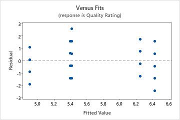
Residuals versus fits plot
Use the residuals versus fits plot to verify the assumption that the residuals are randomly distributed and have constant variance. Ideally, the points should fall randomly on both sides of 0, with no recognizable patterns in the points.
| Pattern | What the pattern may indicate |
|---|---|
| Fanning or uneven spreading of residuals across fitted values | Nonconstant variance |
| Curvilinear | A missing higher-order term |
| A point that is far away from zero | An outlier |
| A point that is far away from the other points in the x-direction | An influential point |
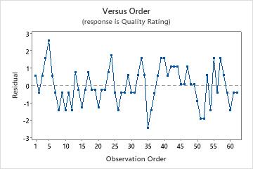
Residuals versus order plot
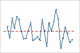
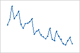
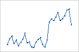
Trend
Shift
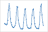
Cycle
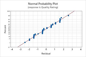
Normal probability plot of the residuals
Use the normal probability plot of the residuals to verify the assumption that the residuals are normally distributed. The normal probability plot of the residuals should approximately follow a straight line.
| Pattern | What the pattern may indicate |
|---|---|
| Not a straight line | Nonnormality |
| A point that is far away from the line | An outlier |
| Changing slope | An unidentified variable |