In This Topic
Transformations

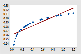
Original

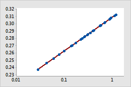
Transformed
For example, in the original scatterplot, the simple regression line does not accurately model the curvature in the data. After the x-scale is transformed using log10, the data values fall along the simple regression line.
When trying to fit curvature in the data, you can also fit a quadratic or cubic model, which adds quadratic or cubic terms to the model. Instead, consider transforming the X or Y variable because you don't have to include additional terms in the model. Adding terms to the model uses additional degrees of freedom, which reduces the degrees available for explaining the variation in the response.
- Log10 of X or Y
- You can choose to transform the Y variable, the X variable, or both. If you are uncertain about which variable to transform, try transforming one variable at a time and then evaluate how well the model fits the data.
- Display logscale for Y variable or X variable
- When you transform the X or Y variable, you can display the logscale for the variable you transform. You may want to display the logscale for the following reasons:
- To view the fitted curve as a straight line, which can make it easier to see how well the regression model fits the data.
- To make it easier to examine data that varies widely in magnitude.
- To conform to industry or company guidelines or preferences.
Display Options
- Display confidence interval
- Display the confidence interval around the fitted regression line. The confidence interval represents a range of likely values for the mean response, given the specified settings of the predictor.
- Display prediction interval
- Display the prediction interval around the fitted regression line. The prediction interval represents a range of likely values for a single new observation, given the specified settings of the predictor. The prediction interval is always wider than the corresponding confidence interval because predicting a single response value is less certain than predicting the mean response value.
- Confidence level
-
Usually, a confidence level of 95% works well. A 95% confidence level indicates that, if you took 100 random samples from the population, the confidence intervals for approximately 95 of the samples would contain the mean response. Similarly, the prediction interval indicates that you can be 95% confident that the interval contains the value of a single new observation. For a given set of data, a lower confidence level produces a narrower interval, and a higher confidence level produces a wider interval.
Title
In Title, you can enter a custom title for the fitted line plot.
