Pareto chart
Minitab provides a Pareto chart of the effects to visualize the results from the coefficient and ANOVA tables. For the terms in the model, this graph allows you to compare the relative magnitude of the effects and to evaluate their statistical significance. Minitab draws the Pareto chart when the model leaves at least 1 degree of freedom for error.
The threshold for statistical significance depends on the significance level (denoted by α or alpha). Unless you use a stepwise selection method, the significance level is 1 minus the confidence level for the analysis. For more information on how to change the confidence level, go to Select the options for Fit Regression Model and Linear Regression. If you use backwards selection or stepwise selection, the significance level is the significance level where Minitab removes a term from the model, known as Alpha to remove. If you use forward selection, the significance level is the significance level where Minitab adds a term to the model, known as Alpha to enter. For more information on the choices for the stepwise methods, go to Perform stepwise regression for Fit Regression Model and Linear Regression.
Residual Plots
- Residuals for Plots
- Specify the type of residuals to display on the residual plots. For more information, go to Which types of residuals are included in Minitab?.
- Regular: Plot the regular raw residuals.
- Standardized: Plot the standardized residuals.
- Deleted: Plot the Studentized deleted residuals.
- Residual Plots
- Use residual plots to examine whether your model meets the assumptions of the analysis. For more information, go to Residual plots in Minitab.
- Individual plots: Select the residual plots that you want to display.
- Histogram of residuals
- Display a histogram of the residuals.
- Normal probability plot of residuals
- Display a normal probability plot of the residuals.
- Residuals versus fits
- Display the residuals versus the fitted values.
- Residuals versus order
- Display the residuals versus the order of the data. The row number for each data point is shown on the x-axis.
- Four in one: Display all four residual plots together in one graph.
- Individual plots: Select the residual plots that you want to display.
- Residuals versus the variables
- Enter one or more variables to plot versus the residuals. You can plot the following types of variables:
- Variables that are already in the current model, to look for curvature in the residuals.
- Important variables that are not in the current model, to determine whether they are related to the response.
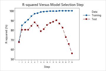
R-squared versus model selection step
When you use Forward selection with validation as the stepwise procedure, Minitab provides a plot of the R2 statistic for the training data set and either the test R2 statistic or the k-fold stepwise R2 statistic for each step in the model selection procedure. The display of the test R2 statistic or the k-fold stepwise R2 statistic depends on whether you use a test data set or k-fold cross-validation.
Interpretation
Use the plot to compare the values of the different R2 statistics at each step. Typically, the model performs well when the R2 statistics are both large. Minitab displays regression statistics for the model from the step that maximizes either the test R2 statistic or the k-fold stepwise R 2 statistic. The plot shows whether any simpler models fit well enough that they can also be good candidates.
In a case where the model is overfit, the test R2 statistic or the k-fold stepwise R2 statistic starts to decrease as terms enter the model. This decrease happens while the corresponding training R2 statistic or R2 statistic for all the data continues to increase. An over-fit model occurs when you add terms for effects that are not important in the population. An overfit model may not be useful for making predictions about the population. If a model is overfit, you can consider models from earlier steps.
The following plot shows test R2 as an example. Initially, the R2 statistics are both close to 70%. For the first few steps, the R2 statistics both tend to increase as terms enter the model. At step 6, the test R2 statistic is about 88%. The maximum value of the test R2 statistic is at step 14 and has a value close to 90%. You can consider whether the improvement in the fit justifies the additional complexity from adding more terms to the model.
After step 14, while the R2 continues to increase, the test R2 does not. The decrease in the test R2 after step 14 indicates that the model is overfit.