In This Topic
Step 1: Investigate alternative trees
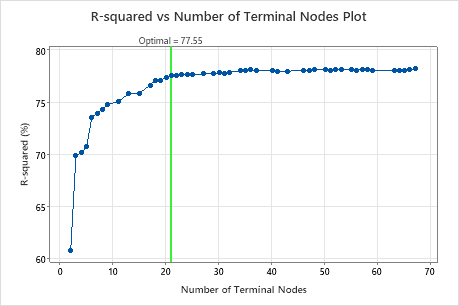
The R-squared vs Number of Terminal Nodes Plot displays the R2 value for each tree. By default, the initial regression tree is the smallest tree with an R2 value within 1 standard error of the value for the tree that maximizes the R2 value. When the analysis uses cross-validation or a test data set, the R2 value is from the validation sample. The values for the validation sample typically level off and eventually start to decline as the tree grows larger.
Click Select Alternative Tree to open an interactive plot that includes a table of model summary statistics. Use the plot to investigate alternative trees with similar performance.
- The tree that Minitab selects is part of a pattern where the criterion improves. One or more trees that have a few more nodes are part of the same pattern. Typically, you want to make predictions from a tree with as much prediction accuracy as possible.
- The tree that Minitab selects is part of a pattern where the criterion is relatively flat. One or more trees with similar model summary statistics have much fewer nodes than the optimal tree. Typically, a tree with fewer terminal nodes gives a clearer picture of how each predictor variable affects the response values. A smaller tree also makes it easier to identify a few target groups for further studies. If the difference in prediction accuracy for a smaller tree is negligible, you can also use the smaller tree to evaluate the relationships between the response and the predictor variables.
Key Result: R-squared vs Number of Terminal Nodes Plot for Tree with 21 Terminal Nodes
The regression tree with 21 terminal nodes has an R2 value of approximately 0.78. This tree has the label "Optimal" because the criterion for the creation of the tree was the smallest tree with an R2 value within 1 standard deviation of the maximum R2 value. Because this chart shows that the R2 values are relatively stable between trees with about 20 nodes to trees with about 70 nodes, the researchers want to look at the performance of some of the even smaller trees that are similar to the tree in the results. Compare the next graph to see results for a tree with 17 nodes.
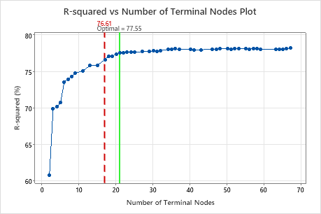
Key Result: R-squared vs Number of Terminal Nodes Plot for Tree with 17 Terminal Nodes
The regression tree with 17 terminal nodes has an R2 value of 0.7661. The tree from the initial results keeps the label "Optimal" when you use Select Alternative Tree to create results for a different tree.
Step 2: Investigate interesting nodes on the tree diagram
After you select a tree, investigate the distinctive terminal nodes on the tree diagram. For example, you might be interested in nodes with large means or with small standard deviations. From the detailed view, you can see the mean, standard deviation, and total counts for each node.
Note
Right-click the tree diagram to perform the following interactions:
- Highlight the 5 nodes with the least variation from the fitted value for the node. These nodes are the optimal nodes.
- Highlight the 5 nodes with the highest means or medians, depending on the criterion for the tree.
- Highlight the 5 nodes with the lowest means or medians, depending on the criterion for the tree.
- Copy the values of the predictors that lead to a node that you select. These values are the node rules.
- Show the Node Split View. This view is helpful when you have a large tree and want to see only which variables split the nodes.
Nodes continue to split until the terminal nodes cannot be split into further groupings. Explore other nodes to see which variables are most interesting.
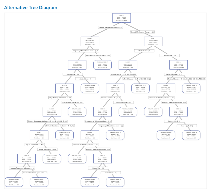
Key Result: Tree Diagram for Tree with 17 Nodes
The tree diagram shows all 4453 cases from the full data set. You can toggle views of the tree between the detailed and node split view.
- Node 2 has the cases where Planned Medication Therapy = 1. This node has 1881 cases. The mean for the node is less than the overall mean. The standard deviation for Node 2 is about 5.4, which is less than the overall standard deviation because a split yields more pure nodes.
- Node 8 has the cases where Planned Medication Therapy = 2. This node has 2572 cases. The mean for the node is more than the overall mean. The standard deviation for Node 8 is about 6.1, which is also less than the overall standard deviation.
Then, Node 2 splits by Frequency of Substance Abuse and Node 8 splits by the Alcohol Use. Terminal Node 17 has the cases for Planned Medication Therapy = 2, Alcohol Use = 1, and Referral Source = 3, 5, 6, 100, 300, 400, 600, 700, or 800. The researchers note that Terminal Node 17 has the highest mean, the smallest standard deviation, and the most cases.
Terminal Node 1 has the smallest mean and a standard deviation of about 4.3. Because the mean of Terminal Node 1 is about 5.9 and the response values cannot be negative, the node statistics suggest that data in Terminal Node 1 are probably right-skewed.
Step 3: Determine the important variables
Use the relative variable importance chart to see which predictors are the most important variables to the tree.
Important variables are a primary or surrogate splitters in the tree. The variable with the highest improvement score is set as the most important variable, and the other variables are ranked accordingly. Relative variable importance standardizes the importance values for ease of interpretation. Relative importance is defined as the percent improvement with respect to the most important predictor.
Relative variable importance values range from 0% to 100%. The most important variable always has a relative importance of 100%. If a variable is not in the tree, that variable is not important.
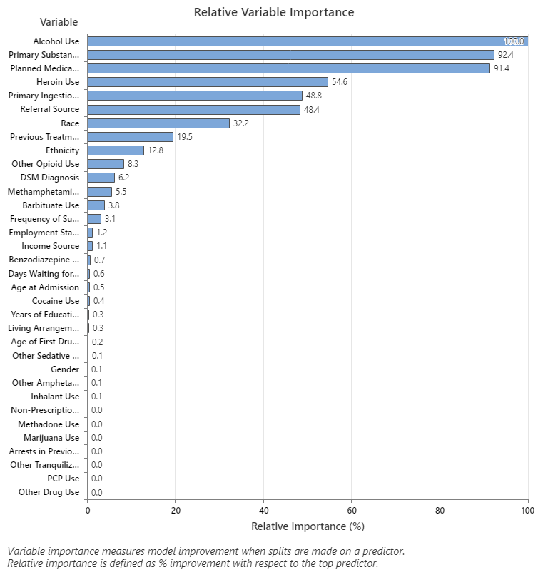
Key Result: Relative Variable Importance
- Primary Substance of Abuse and Planned Medication Therapy are about 92% as important as Alcohol Use.
- Heroin Use is about 55% as important as Alcohol Use.
- Primary Ingestion Route of Sub and Referral Source are about 48% as important as Alcohol Use.
Although these results include 33 variables with positive importance, the relative rankings provide information about how many variables to control or monitor for a certain application. Steep drops in the relative importance values from one variable to the next variable can guide decisions about which variables to control or monitor. For example, in these data, the three most important variables have importance values that are relatively close together before a drop of almost 40% in relative importance to the next variable. Similarly, three variables have similar importance values near 50%. You can remove variables from different groups and redo the analysis to evaluate how variables in various groups affect the prediction accuracy values in the model summary table.