A clean room engineer analyzes a response surface design to determine how seal time, temperature, and pressure affect the seal quality of the sealed trays. The response is binary—whether the seal is intact or not—in a sample of 800 tray seals.
The engineer collects data and analyzes the design to determine which factors impact seal strength.
- Open the sample data, TraySeal.MWX.
- Choose .
- In Event name, enter Event.
- In Number of events, enter Sealed.
- In Number of trials, enter Samples.
- Click Terms.
- Under Include the following terms, choose Full quadratic.
- Click OK.
- Click Graphs.
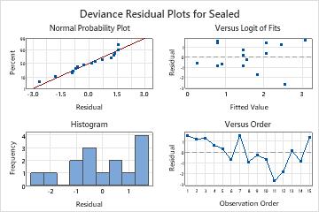
- Under Residual Plots, select Four in one.
- Click OK in each dialog box.
Interpret the results
In the Analysis of Variance table, the p-values for Temperature, Pressure and Temperature*Temperature are significant. The engineer can consider reducing the model to remove the terms that are not significant. For more information, go to Model reduction.
The Deviance R2 value shows that the model explains 97.47% of the total deviance in the response, which indicates that the model fits the data well.
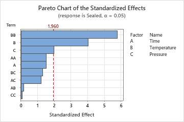
The Pareto plot of the effects allow you to visually identify the important effects and compare the relative magnitude of the various effects. In addition, you can see that the largest effect is Temperature*Temperature (BB) because it extends the farthest.
Response Information
| Variable | Value | Count | Event Name |
|---|---|---|---|
| Sealed | Event | 9637 | Event |
| Non-event | 2363 | ||
| Samples | Total | 12000 |
Coded Coefficients
| Term | Coef | SE Coef | VIF |
|---|---|---|---|
| Constant | 3.021 | 0.384 | |
| Time | 0.210 | 0.139 | 18.53 |
| Temperature | 0.641 | 0.159 | 19.53 |
| Pressure | 0.420 | 0.211 | 70.48 |
| Time*Time | -0.0735 | 0.0482 | 1.01 |
| Temperature*Temperature | 0.2988 | 0.0517 | 1.17 |
| Pressure*Pressure | -0.0022 | 0.0277 | 70.24 |
| Time*Temperature | -0.0092 | 0.0505 | 1.14 |
| Time*Pressure | 0.0417 | 0.0342 | 18.12 |
| Temperature*Pressure | -0.0521 | 0.0396 | 19.24 |
Odds Ratios for Continuous Predictors
| Unit of Change | Odds Ratio | 95% CI | |
|---|---|---|---|
| Time | 1.0 | * | (*, *) |
| Temperature | 25.0 | * | (*, *) |
| Pressure | 7.5 | * | (*, *) |
Model Summary
| Deviance R-Sq | Deviance R-Sq(adj) | AIC | AICc | BIC |
|---|---|---|---|---|
| 97.47% | 96.50% | 140.64 | 195.64 | 147.72 |
Goodness-of-Fit Tests
| Test | DF | Chi-Square | P-Value |
|---|---|---|---|
| Deviance | 5 | 23.40 | 0.000 |
| Pearson | 5 | 23.88 | 0.000 |
| Hosmer-Lemeshow | 5 | 7.47 | 0.188 |
Analysis of Variance
| Source | DF | Adj Dev | Adj Mean | Chi-Square | P-Value |
|---|---|---|---|---|---|
| Model | 9 | 903.478 | 100.386 | 903.48 | 0.000 |
| Time | 1 | 2.303 | 2.303 | 2.30 | 0.129 |
| Temperature | 1 | 16.388 | 16.388 | 16.39 | 0.000 |
| Pressure | 1 | 3.966 | 3.966 | 3.97 | 0.046 |
| Time*Time | 1 | 2.331 | 2.331 | 2.33 | 0.127 |
| Temperature*Temperature | 1 | 34.012 | 34.012 | 34.01 | 0.000 |
| Pressure*Pressure | 1 | 0.006 | 0.006 | 0.01 | 0.937 |
| Time*Temperature | 1 | 0.033 | 0.033 | 0.03 | 0.856 |
| Time*Pressure | 1 | 1.490 | 1.490 | 1.49 | 0.222 |
| Temperature*Pressure | 1 | 1.731 | 1.731 | 1.73 | 0.188 |
| Error | 5 | 23.404 | 4.681 | ||
| Total | 14 | 926.882 |
Regression Equation in Uncoded Units
| P(Event) | = | exp(Y')/(1 + exp(Y')) |
|---|
| Y' | = | 17.77 + 0.348 Time - 0.1918 Temperature + 0.1146 Pressure - 0.0735 Time*Time + 0.000478 Temperature*Temperature - 0.000039 Pressure*Pressure - 0.00037 Time*Temperature + 0.00556 Time*Pressure - 0.000278 Temperature*Pressure |
|---|
Fits and Diagnostics for Unusual Observations
| Obs | Observed Probability | Fit | Resid | Std Resid | |
|---|---|---|---|---|---|
| 1 | 0.7113 | 0.6856 | 1.5722 | 4.45 | R |
| 3 | 0.9025 | 0.8879 | 1.3370 | 2.50 | R |
| 7 | 0.9675 | 0.9565 | 1.5927 | 2.17 | R |
| 8 | 0.6737 | 0.6884 | -0.8891 | -2.44 | R |
| 10 | 0.5550 | 0.5660 | -0.6265 | -2.07 | R |
| 11 | 0.9025 | 0.9281 | -2.6700 | -4.20 | R |
| 12 | 0.8413 | 0.8633 | -1.7806 | -3.54 | R |
| 15 | 0.7113 | 0.6892 | 1.3592 | 3.64 | R |