In This Topic
- Probability density function
- Cumulative distribution function
- Inverse cumulative probability
- Beta distribution
- Binomial distribution
- Cauchy distribution
- Chi-square distribution
- Discrete distribution
- Exponential distribution
- F-distribution
- Gamma distribution
- Geometric distribution
- Hypergeometric distribution
- Integer distribution
- Normal distribution
- Laplace distribution
- Largest extreme value distribution
- Logistic distribution
- Loglogistic distribution
- Lognormal distribution
- Negative binomial distribution
- Poisson distribution
- Smallest extreme value distribution
- t-distribution
- Triangular distribution
- Uniform distribution
- Weibull distribution
Probability density function
- For continuous distributions, the probability that X has values in an interval (a, b) is precisely the area under its PDF in the interval (a, b).
- For discrete distributions, the probability that X has values in an interval (a, b) is exactly the sum of the PDF (also called the probability mass function) of the possible discrete values of X in (a, b).
Cumulative distribution function
- For continuous distributions, the CDF gives the area under the probability density function, up to the x-value that you specify.
- For discrete distributions, the CDF gives the cumulative probability for x-values that you specify.
Inverse cumulative probability
For a number p in the closed interval [0,1], the inverse cumulative distribution function (ICDF) of a random variable X determines, where possible, a value x such that the probability of X ≤ x is greater than or equal to p.
- The ICDF for continuous distributions
-
The ICDF is the value that is associated with an area under the probability density function. The ICDF is the reverse of the cumulative distribution function (CDF), which is the area that is associated with a value.
For all continuous distributions, the ICDF exists and is unique if 0 < p < 1.
- When the probability density function (PDF) is positive for the entire real number line (for example, the normal PDF), the ICDF is not defined for either p = 0 or p = 1.
- When the PDF is positive for all values that are greater than some value (for example, the chi-square PDF), the ICDF is defined for p = 0 but not for p = 1.
- When the PDF is positive only on an interval (for example, the uniform PDF), the ICDF is defined for p = 0 and p = 1.
- When the ICDF is not defined, Minitab returns a missing value (*) for the result.
- The ICDF for discrete distributions
- The ICDF is more complicated for discrete distributions than it is for continuous distributions. When you calculate the CDF for a binomial with, for example, n = 5 and p = 0.4, there is no value x such that the CDF is 0.5. For x = 1, the CDF is 0.3370. For x = 2, the CDF increases to 0.6826.
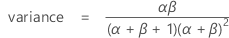
Beta distribution
The beta distribution is often used to represent processes with natural lower and upper limits.
Formula
The probability density function (PDF) is:

Notation
| Term | Description |
|---|---|
| α | shape parameter 1 |
| β | shape parameter 2 |
| Γ | gamma function |
| a | lower limit |
| b | upper limit |
When a = 0, b = 1,
the PDF is:

Binomial distribution
The binomial distribution is used to represent the number of events that occurs within n independent trials. Possible values are integers from zero to n.
Formula
mean = np
variance = np(1 – p)
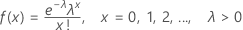
The probability mass function (PMF) is:

Where  equals
  .
.
In general, you can calculate k! as 
Notation
| Term | Description |
|---|---|
| n | number of trials |
| x | number of events |
| p | event probability |
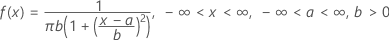
Cauchy distribution
The Cauchy distribution is symmetric around zero, but the tails approach zero less quickly than do those of the normal distribution.
Formula
The probability density function (PDF) is:
Notation
| Term | Description |
|---|---|
| a | location parameter |
| b | scale parameter |
| π | Pi (~3.142) |
Note
If you do not specify values, Minitab uses a = 0 and b = 1.
Chi-square distribution
If X has a standard normal distribution, X2 has a chi-square distribution with one degree of freedom, allowing it to be a commonly used sampling distribution.
The sum of n independent X2 variables (where X has a standard normal distribution) has a chi-square distribution with n degrees of freedom. The shape of the chi-square distribution depends on the number of degrees of freedom.
Formula
The probability density function (PDF) is:
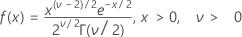
mean = v
variance = 2v
Notation
| Term | Description |
|---|---|
| ν | degrees of freedom |
| Γ | gamma function |
| e | base of the natural logarithm |
Discrete distribution
A discrete distribution is one that you define yourself. For example, suppose you are interested in a distribution made up of three values −1, 0, 1, with probabilities of 0.2, 0.5, and 0.3, respectively. If you enter the values into columns of a worksheet, then you can use these columns to generate random data or to calculate probabilities.
| Value | Prob |
|---|---|
| −1 | 0.2 |
| 0 | 0.5 |
| 1 | 0.3 |
Exponential distribution
The exponential distribution can be used to model time between failures, such as when units have a constant, instantaneous rate of failure (hazard function). The exponential distribution is a special case of the Weibull distribution and the gamma distribution.
Formula
The probability density function (PDF) is:

The cumulative distribution function (CDF) is:

mean = θ + λ
variance = θ2
Notation
| Term | Description |
|---|---|
| θ | scale parameter |
| λ | threshold parameter |
| exp | base of the natural logarithm |
Note
Some references use 1 / θ for a parameter.
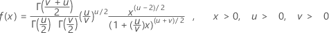
F-distribution
The F-distribution is also known as the variance-ratio distribution and has two types of degrees of freedom: numerator degrees of freedom and denominator degrees of freedom. It is the distribution of the ratio of two independent random variables with chi-square distributions, each divided by its degrees of freedom.
Formula
The probability density function (PDF) is:


Notation
| Term | Description |
|---|---|
| Γ | gamma function |
| u | numerator degrees of freedom |
| v | denominator degrees of freedom |
Gamma distribution
The gamma distribution is often used to model positively skewed data.
Formula
The probability density function (PDF) is:
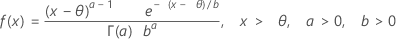
mean = ab + θ
variance = ab2
Notation
| Term | Description |
|---|---|
| a | shape parameter (when a = 1, the gamma PDF is the same as the exponential PDF) |
| b | scale parameter |
| θ | threshold parameter |
| Γ | gamma function |
| e | base of the natural logarithm |
Note
Some references use 1/ b for a parameter.
Geometric distribution
The discrete geometric distribution applies to a sequence of independent Bernoulli experiments with an event of interest that has probability p.
Formula
If the random variable X is the total number of trials necessary to produce one event with probability p, then the probability mass function (PMF) of X is given by:
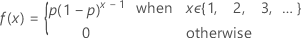
and X exhibits the following properties:

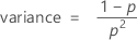
If the random variable Y is the number of nonevents that occur before the first event (with probability p) is observed, then the probability mass function (PMF) of Y is given by:
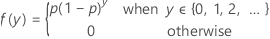
and Y exhibits the following properties:


Notation
| Term | Description |
|---|---|
| X | number of trials to produce one event, Y + 1 |
| Y | number of nonevents that occur before the first event |
| p | probability that an event occurs on each trial |
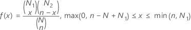
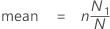
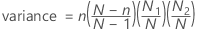
Hypergeometric distribution
The hypergeometric distribution is used for samples drawn from small populations, without replacement. For example, you have a shipment of N televisions, where N1 are good (successes) and N2 are defective (failure). If you sample n televisions of N at random, without replacement, you can find the probability that exactly x of the n televisions are good.
Formula
The probability mass function (PMF) is:
Notation
| Term | Description |
|---|---|
| N | N1 + N2 = population size |
| N1 | number of events in the population |
| N2 | number of non-events in the population |
| n | sample size |
| x | number of events in the sample |
Integer distribution
The integer distribution is a discrete uniform distribution on a set of integers. Each integer has equal probability of occurring.
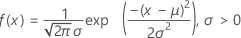
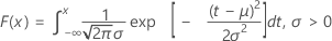
Normal distribution
The normal distribution (also called Gaussian distribution) is the most used statistical distribution because of the many physical, biological, and social processes that it can model.
Formula
The probability density function (PDF) is:
The cumulative distribution function (CDF) is:
mean = μ
variance = σ 2
standard deviation = σ
Notation
| Term | Description |
|---|---|
| exp | base of the natural logarithm |
| π | Pi (~3.142) |
Laplace distribution
The Laplace distribution is used when the distribution is more peaked than a normal distribution.
Formula
The probability density function (PDF) is:

mean = a
variance = 2b2
Notation
| Term | Description |
|---|---|
| a | location parameter |
| b | scale parameter |
| e | base of natural logarithm |
Largest extreme value distribution
Use the largest extreme value distribution to model the largest value from a distribution. If you have a sequence of exponential distributions, and X(n) is the maximum of the first n, then X(n) – ln(n) converges in distribution to the largest extreme value distribution. Thus, for large values of n, the largest extreme value distribution is a good approximation to the distribution of X(n) – ln(n).
Formula
The probability density function (PDF) is:

The cumulative distribution function (CDF) is:

mean = μ + γσ
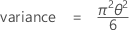
variance = π 2 σ 2 / 6
Notation
| Term | Description |
|---|---|
| σ | scale parameter |
| μ | location parameter |
| γ | Euler constant (~0.57722) |
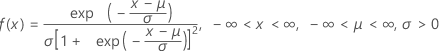
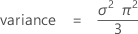
Logistic distribution
A continuous distribution that is symmetric, similar to the normal distribution, but with heavier tails.
Formula
The probability density function (PDF) is:
The cumulative distribution function (CDF) is:

mean = μ
Notation
| Term | Description |
|---|---|
| μ | location parameter |
| σ | scale parameter |
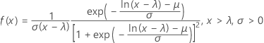
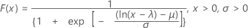
Loglogistic distribution
A variable x has a loglogistic distribution with threshold λ if Y = log (x – λ) has a logistic distribution.
Formula
The probability density function (PDF) is:
The cumulative distribution function (CDF) is:
when σ < 1:

when σ < 1/2:

Notation
| Term | Description |
|---|---|
| μ | location parameter |
| σ | scale parameter |
| λ | threshold parameter |
| Γ | gamma function |
| exp | base of the natural logarithm |
Lognormal distribution
A variable x has a lognormal distribution if log(x – λ ) has a normal distribution.
Formula
The probability density function (PDF) is:

The cumulative distribution function (CDF) is:


Notation
| Term | Description |
|---|---|
| μ | location parameter |
| σ | scale parameter |
| λ | threshold parameter |
| π | Pi (~3.142) |
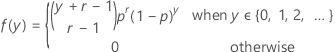
Negative binomial distribution
The discrete negative binomial distribution applies to a series of independent Bernoulli experiments with an event of interest that has probability p.
Formula
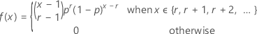

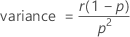
If the random variable Y is the number of nonevents that occur before you observe the r events, which each have probability p, then the probability mass function (PMF) of Y is given by:
and Y exhibits the following properties:


Note
This negative binomial distribution is also known as the Pascal distribution.
Notation
| Term | Description |
|---|---|
| X | Y + r |
| r | number of events |
| p | probability of an event |
Poisson distribution
The Poisson distribution is a discrete distribution that models the number of events based on a constant rate of occurrence. The Poisson distribution can be used as an approximation to the binomial when the number of independent trials is large and the probability of success is small.
Formula
The probability mass function (PMF) is:
mean = λ
variance = λ
Notation
| Term | Description |
|---|---|
| e | base of the natural logarithm |
Smallest extreme value distribution
Use the smallest extreme value distribution to model the smallest value from a distribution. If Y follows the Weibull distribution, then log(Y) follows the smallest extreme value distribution.
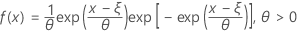
Formula
The probability density function (PDF) is:
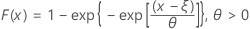
The cumulative distribution function (CDF) is:

Notation
| Term | Description |
|---|---|
| ξ | location parameter |
| θ | scale parameter |
| e | base of the natural logarithm |
| v | Euler constant (~0.57722) |
t-distribution
- Creating confidence intervals of the population mean from a normal distribution when the variance is unknown.
- Determining whether two sample means from normal populations with unknown but equal variances are significantly different.
- Testing the significance of regression coefficients.
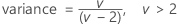
Formula

mean = 0, when ν > 0
Notation
| Term | Description |
|---|---|
| Γ | gamma function |
| v | degrees of freedom |
| π | Pi (~3.142) |
Triangular distribution
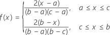
The PDF of the triangular distribution has a triangular shape.
Formula
The probability density function (PDF) is:


Notation
| Term | Description |
|---|---|
| a | lower endpoint |
| b | upper endpoint |
| c | mode (location where the PDF peaks) |
Uniform distribution
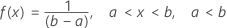
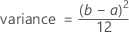
The uniform distribution characterizes data over an interval uniformly, with a as the smallest value and b as the largest value.
Formula
The probability density function (PDF) is:

Notation
| Term | Description |
|---|---|
| a | lower endpoint |
| b | upper endpoint |
Weibull distribution
The Weibull distribution is useful to model product failure times.
Formula
The probability density function (PDF) is:

The cumulative distribution function (CDF) is:


Notation
| Term | Description |
|---|---|
| α | scale parameter |
| β | shape parameter, when β = 1 the Weibull PDF is the same as the exponential PDF |
| λ | threshold parameter |
| Γ | gamma function |
| exp | base of the natural logarithm |
Note
Some references use 1/α as a parameter.