In This Topic
Step 1: Look for outliers and sudden shifts
Use process knowledge to determine whether unusual observations or shifts indicate errors or a real change in the process.
Outliers
Look for unusual observations, also called outliers. Outliers can have a disproportionate effect on time series models and produce misleading results. Try to identify the cause of any outliers and correct any data-entry errors or measurement errors. Consider removing data values that are associated with abnormal, one-time events, which are also called special causes.
Sudden shifts
Look for sudden shifts in the series or sudden changes to trends. Try to identify the cause of such changes.
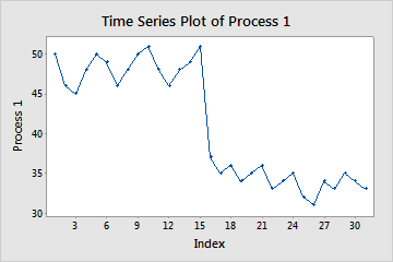
For example, the following time series plot shows a drastic shift in the cost of a process after 15 months. You should investigate the reason for the shift.
Step 2: Look for trends
A trend is a long-term increase or decrease in the data values. A trend can be linear, or it can exhibit some curvature. If your data exhibit a trend, you can use a time series analysis to model the data and generate forecasts. For more information on which analysis to use, go to Which time series analysis should I use?.
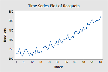
The following time series plot shows a clear upward trend. There may also be a slight curve in the data, because the increase in the data values seems to accelerate over time. If there is curvature, then a quadratic model is the most appropriate.
Step 3: Look for seasonal patterns or cyclic movements
A seasonal pattern is a rise and fall in the data values that repeats regularly over the same time period. For example, orders at an auto parts store are low each Monday, increase during the week, and peak each Friday. Seasonal patterns always have a fixed and known period. In contrast, cyclic movements are cycles of rising and falling data values that do not repeat at regular intervals. Typically, cyclic movements are longer and more variable than seasonal patterns.
You can use a time series analysis to model patterns and generate forecasts. For more information on which analysis to use, go to Which time series analysis should I use?.
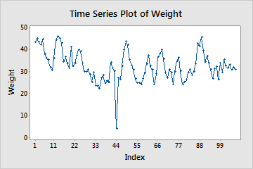
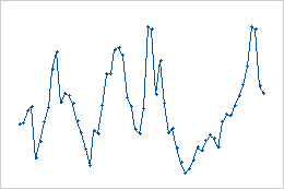
- Seasonal pattern
- These data show a seasonal pattern. The pattern repeats every 12 months.
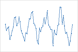
- Cyclic movements
- These data show cyclic movements. The cycles do not repeat at regular intervals and do not have the same shape.
- Random variation
- These data show random variation. There are no patterns or cycles.

Step 4: Assess whether seasonal changes are additive or multiplicative
If the magnitude of the seasonal changes is constant, then the seasonal changes are additive. If the magnitude of the seasonal changes is greater when the data values are greater, then the seasonal changes are multiplicative. The extra variability can make multiplicative seasonal changes harder to forecast accurately.
If the pattern is not obvious, and you have trouble choosing between the additive and multiplicative procedures to model your data, you can try both and choose the one with smaller accuracy measures. For more information, go to Which time series analysis should I use?.
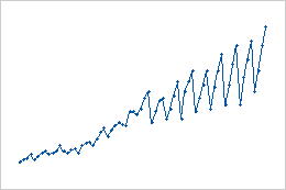
- Additive changes
- In this example of additive seasonal changes, the data values tend to increase over time, but the magnitude of the seasonal change remains the same.
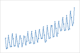
- Multiplicative changes
- In this example of multiplicative seasonal changes, the magnitude of the seasonal change increases over time as the data values increase.