A buyer for a t-shirt shop wants to compare the proportion of t-shirts of each size that are sold to the proportion that were ordered. The buyer counts the number of t-shirts of each size that are sold in a week.
The buyer performs a chi-square goodness-of-fit test to determine whether the proportions of t-shirt sizes sold are consistent with the proportion of t-shirt sizes ordered.
- Open the sample data, TshirtSales.MWX.
- Choose .
- In Observed counts, enter Counts.
- In Category names (optional), enter Size.
- Under Test, select Specific proportions, and enter Proportions
- Click OK.
Interpret the results
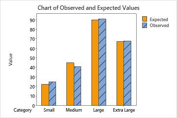
- 25 small shirts were sold, while 22.5 were expected to be sold.
- 41 medium shirts were sold, while 45 were expected to be sold.
- 91 large shirts were sold, while 90 were expected to be sold.
- 68 extra-large shirts were sold, while 67.5 were expected to be sold.
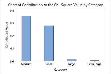
The largest difference between observed and expected sales is in the medium category. Consequently, this category has the largest contribution to the chi-square statistic, 0.355.
The overall chi-square statistic is 0.648 and has a p-value of 0.885. Because the p-value is greater than the significance level of 0.05, the buyer fails to reject the null hypothesis. The buyer concludes that there is not a significant difference between the observed t-shirt sales and the expected t-shirt sales.
Observed and Expected Counts
| Category | Observed | Test Proportion | Expected | Contribution to Chi-Square |
|---|---|---|---|---|
| Small | 25 | 0.1 | 22.5 | 0.277778 |
| Medium | 41 | 0.2 | 45.0 | 0.355556 |
| Large | 91 | 0.4 | 90.0 | 0.011111 |
| Extra Large | 68 | 0.3 | 67.5 | 0.003704 |
Chi-Square Test
| N | DF | Chi-Sq | P-Value |
|---|---|---|---|
| 225 | 3 | 0.648148 | 0.885 |