α (alpha)
The significance level (denoted as α or alpha) is the maximum acceptable level of risk for rejecting the null hypothesis when the null hypothesis is true (type I error). Alpha is also interpreted as the power of the test when the null hypothesis (H0) is true. Usually, you choose the significance level before you analyze the data. The default significance level is 0.05.
Interpretation
Use the significance level to minimize the power value of the test when the null hypothesis (H0) is true. Higher values for the significance level give the test more power, but also increase the chance of making a type I error, which is rejecting the null hypothesis when it is true.
Length of observation
Poisson processes count occurrences of a certain event or property on a specific observation range, which can represent things such as time, area, volume, and number of items. The length of observation represents the magnitude, duration, or size of each observation range.
Interpretation
Minitab uses the length of observation to convert the rate of occurrence into a form that is best for your situation.
For example, if each sample observation counts the number of events in a year, a length of 1 represents a yearly rate of occurrence, and a length of 12 represents a monthly rate of occurrence.
- The total occurrences is 122 because the inspectors find 122 defects.
- The sample size (N) is 50 because the inspectors sample 50 boxes.
- To determine the number of defects per towel, inspectors use a length of observation of 10 because each box contains 10 towels. To determine the number of defects per box, inspectors use a length of observation of 1.
- The rate of occurrence is (Total occurrences / N) / (length of observation) = (122/50) / 10 = 0.244. So, on average, each towel has 0.244 defects.
Comparison rate
The comparison rate is the value you want to compare to the hypothesized rate.
Interpretation
Minitab calculates the comparison rate. The difference between the comparison rate and the hypothesized rate is the minimum difference for which you can achieve the specified level of power for each sample size. Larger sample sizes enable the test to detect smaller differences. You want to detect the smallest difference that has practical consequences for your application.
To more fully investigate the relationship between the sample size and the comparison rate at a given power, use the power curve.
Sample size
The sample size is the total number of observations in the sample.
Interpretation
Use the sample size to estimate how many observations you need to obtain a certain power value for the hypothesis test at a specific difference.
Minitab calculates how large your sample must be for a test with your specified power to detect the difference between the hypothesized rate and comparison rate. Because sample sizes are whole numbers, the actual power of the test might be slightly greater than the power value that you specify.
If you increase the sample size, the power of the test also increases. You want enough observations in your sample to achieve adequate power. But you don't want a sample size so large that you waste time and money on unnecessary sampling or detect unimportant differences to be statistically significant.
To more fully investigate the relationship between the sample size and the difference at a given power, use the power curve.
Power
The power of a hypothesis test is the probability that the test correctly rejects the null hypothesis. The power of a hypothesis test is affected by the sample size, the difference, the variability of the data, and the significance level of the test.
For more information, go to What is power?.
Interpretation
Minitab calculates the power of the test based on the specified comparison rate and sample size. A power value of 0.9 is usually considered adequate. A value of 0.9 indicates you have a 90% chance of detecting a difference between the hypothesized rate and the population comparison rate when a difference actually exists. If a test has low power, you might fail to detect a difference and mistakenly conclude that none exists. Usually, when the sample size is smaller or the difference is smaller, the test has less power to detect a difference.
If you enter a comparison rate and a power value for the test, then Minitab calculates how large your sample must be. Minitab also calculates the actual power of the test for that sample size. Because sample sizes are whole numbers, the actual power of the test might be slightly greater than the power value that you specify.
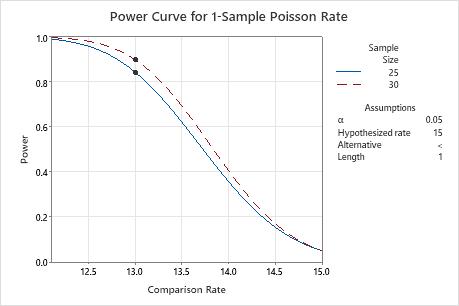
Power curve
The power curve plots the power of the test versus the comparison rate.
Interpretation
Use the power curve to assess the appropriate sample size or power for your test.
The power curve represents every combination of power and comparison rate for each sample size when the significance level is held constant. Each symbol on the power curve represents a calculated value based on the values that you enter. For example, if you enter a sample size and a power value, Minitab calculates the corresponding comparison proportion and displays the calculated value on the graph.
Examine the values on the curve to determine the difference between the comparison rate and the hypothesized rate that can be detected at a certain power value and sample size. A power value of 0.9 is usually considered adequate. However, some practitioners consider a power value of 0.8 to be adequate. If a hypothesis test has low power, you might fail to detect a difference that is practically significant. If you increase the sample size, the power of the test also increases. You want enough observations in your sample to achieve adequate power. But you don't want a sample size so large that you waste time and money on unnecessary sampling or detect unimportant differences to be statistically significant. If you decrease the size of the difference that you want to detect, the power also decreases.
In this graph, the power curve for a sample size of 25 shows that the test has a power of approximately 0.84 for a comparison rate of 13. For a sample size of 30, the power curve shows that the test has a power of approximately 0.9 for a comparison rate of 13. As the comparison rate approaches the hypothesized rate (15 in this graph), the power of the test decreases and approaches α (also called the significance level), which is 0.05 for this analysis.