In This Topic
Null hypothesis and alternative hypothesis
- Null hypothesis
- The null hypothesis states that all the data values come from the same normal distribution.
- Alternative hypothesis
- The alternative hypothesis states that either the smallest or largest data value is an outlier.
Significance level
The significance level (denoted as α or alpha) is the maximum acceptable level of risk for rejecting the null hypothesis when the null hypothesis is true (type I error). The default value is 0.05.
Interpretation
Use the significance level to decide whether to reject or fail to reject the null hypothesis (H0). If the probability that an event occurs is less than the significance level, the usual interpretation is that the results are statistically significant, and you reject H0.
- Choose a higher significance level, such as 0.10, to be more certain that you detect any difference that possibly exists. For example, a quality engineer compares the stability of new ball bearings with the stability of current bearings. The engineer must be highly certain that the new ball bearings are stable because unstable ball bearings could cause a disaster. The engineer chooses a significance level of 0.10 to be more certain of detecting any possible difference in stability of the ball bearings.
- Choose a lower significance level, such as 0.01, to be more certain that you detect only a difference that actually exists. For example, a scientist at a pharmaceutical company must be very certain about a claim that the company's new drug significantly reduces symptoms. The scientist chooses a significance level of 0.001 to be more certain that any significant difference in symptoms does exist.
N
The sample size (N) is the total number of observations in the sample.
Interpretation
The sample size affects the power of the test.
Usually, a larger sample size gives the test more power to detect an outlier. For more information, go to What is power?.
Mean
The mean is the average of the data, which is the sum of all the observations divided by the number of observations.
Interpretation
Use the mean to describe the sample with a single value that represents the center of the data. Many statistical analyses use the mean as a standard measure of the center of the distribution of the data.
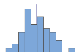
Symmetric
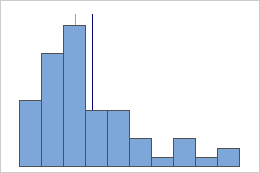
Not symmetric
For the symmetric distribution, the mean (blue line) and median (orange line) are so similar that you can't easily see both lines. But the non-symmetric distribution is skewed to the right.
StDev
The standard deviation is the most common measure of dispersion, or how spread out the data are about the mean. The symbol σ (sigma) is often used to represent the standard deviation of a population, while s is used to represent the standard deviation of a sample. Variation that is random or natural to a process is often referred to as noise.
Because the standard deviation is in the same units as the data, it is usually easier to interpret than the variance.
Interpretation
Use the standard deviation to determine how spread out the data are from the mean. A higher standard deviation value indicates greater spread in the data. A good rule of thumb for a normal distribution is that approximately 68% of the values fall within one standard deviation of the mean, 95% of the values fall within two standard deviations, and 99.7% of the values fall within three standard deviations.
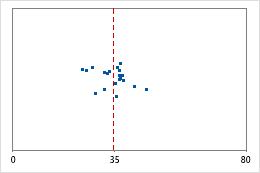
Hospital 1
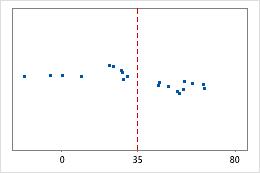
Hospital 2
Hospital discharge times
Administrators track the discharge time for patients who are treated in the emergency departments of two hospitals. Although the average discharge times are about the same (35 minutes), the standard deviations are significantly different. The standard deviation for hospital 1 is about 6. On average, a patient's discharge time deviates from the mean (dashed line) by about 6 minutes. The standard deviation for hospital 2 is about 20. On average, a patient's discharge time deviates from the mean (dashed line) by about 20 minutes.
Maximum
The maximum is the largest data value.
In these data, the maximum is 19.
| 13 | 17 | 18 | 19 | 12 | 10 | 7 | 9 | 14 |
Interpretation
Use the maximum to identify a possible outlier or a data-entry error. One of the simplest ways to assess the spread of your data is to compare the minimum and maximum. If the maximum value is very high, even when you consider the center, the spread, and the shape of the data, investigate the cause of the extreme value.
Minimum
The minimum is the smallest data value.
In these data, the minimum is 7.
| 13 | 17 | 18 | 19 | 12 | 10 | 7 | 9 | 14 |
Interpretation
Use the minimum to identify a possible outlier or a data-entry error. One of the simplest ways to assess the spread of your data is to compare the minimum and maximum. If the minimum value is very low, even when you consider the center, the spread, and the shape of the data, investigate the cause of the extreme value.
Outlier
An outlier is an unusually large or small observation. Try to identify the cause of any outliers. Correct any data–entry errors or measurement errors. Consider removing data values for abnormal, one-time events (also called special causes).
Row
The row in the worksheet that contains the outlier. Minitab displays this value only when an outlier exists.
x[i] and x[N-i]
When you use one of Dixon's ratio tests, Minitab displays more observations in the test table, in addition to the minimum and maximum. The value in the brackets indicates the size of the observation relative to the other values. For example, x[2] denotes the 2nd smallest observation and x[N-1] denotes the 2nd largest observation.
G
Grubbs' test statistic (G) is the difference between the sample mean and either the smallest or largest data value, divided by the standard deviation. Minitab uses Grubbs' test statistic to calculate the p-value, which is the probability of rejecting the null hypothesis when it is true.
P
The p-value is a probability that measures the evidence against the null hypothesis. A smaller p-value provides stronger evidence against the null hypothesis.
Interpretation
Use the p-value to determine whether an outlier exists.
- P-value ≤ α: An outlier exists (Reject H0)
- If the p-value is less than or equal to the significance level, the decision is to reject the null hypothesis and conclude that an outlier exists. Try to identify the cause of any outliers. Correct any data–entry errors or measurement errors. Consider removing data values that are associated with abnormal, one-time events (special causes).
- P-value > α: You cannot conclude an outlier exists (Fail to reject H0)
- If the p-value is greater than the significance level, the decision is to fail to reject the null hypothesis because you do not have enough evidence to conclude that an outlier exists. You should make sure that your test has enough power to detect an outlier. For more information, go to Increase power.
Outlier plot
An outlier plot is similar to an individual plot. Use the outlier plot to visually identify an outlier in the data. If an outlier exists, Minitab represents it on the plot as a red square. Try to identify the cause of any outliers. Correct any data–entry errors or measurement errors. Consider removing data values for abnormal, one-time events (also called special causes).
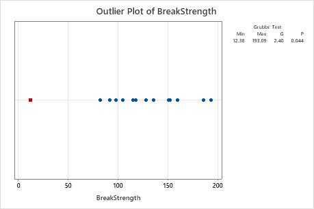
In these results, the smallest value, 12.38, is an outlier.