一家发动机工厂的一名质量工程师想要对两家供应商的活塞进行双峰测试。该工程师随机测量了每个供应商提供的 100 个活塞样本的长度。
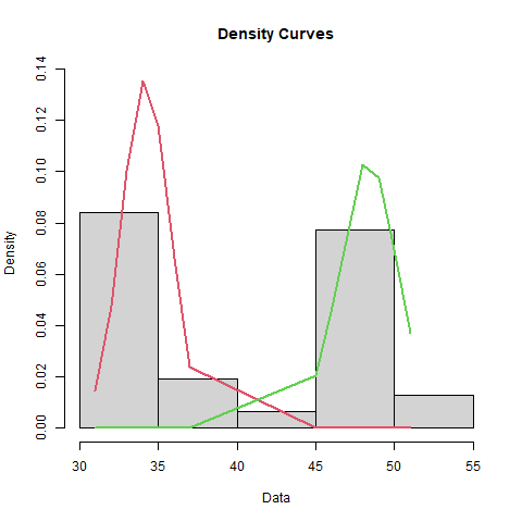
该脚本使用 R 的 diptest 包来测试数据是否为单峰。如果检验拒绝单峰数据的原假设,则脚本假定数据是两个正态分布的混合。该脚本使用 R 的 mixtools 包来显示两个正态分布的描述性统计量和密度曲线。
示例 R 脚本演示了集成的以下功能:
- 将 Minitab 工作表中的单个列作为输入传递。
- 添加表标题。
- 为表添加列标签。
- 将表发送到 Minitab 输出窗格。
- 创建一个图形,并将该图形发送到 Minitab 输出窗格。
使用以下文件执行本节中的步骤:
| 文件 | 说明 |
|---|---|
| bimodal.R | 一个脚本, R 它从 Minitab 工作表中获取列,检验单峰性,并在数据不是单峰时生成两个正态分布混合的结果。 |
以下 .ZIP 文件提供了本指南中引用的所有文件:r_guide_files.zip。
预修课程
-
以下示例中的 R 脚本需要以下 R 包:
- mtbr
- 集成 Minitab 和 R 的 R 包。在该示例中,此模块中的函数将 R 结果发送到 Minitab。有关如何安装 Minitab 软件 R 包的信息,请转至 步骤 2: 安装 mtbr。
- mixtools
- R 脚本用于为正态分布混合创建输出的包。
- diptest
- R 脚本用于测试数据是否为单峰的包。
install.packages("mixtools")如需安装 R 包的帮助,请咨询贵组织的技术支持部门。Minitab 技术支持无法协助安装 R 包。
运行示例的步骤
- 确保已安装所需模块:mtbr。
- 将 R 脚本文件 bimodal.R 保存到 Minitab 默认文件位置。 有关 Minitab 在何处查找 R 脚本文件的更多信息,请转到 Minitab 的 R 文件的默认文件夹。
- 打开样本数据集过程能源成本.MWX。
-
在 Minitab 命令行窗格中,输入
RSCR "bimodal.R" "Process 1"。 - 选择 运行。
bimodal.R
# Load the necessary libraries
#Original code by Valentina Tillman
library(mixtools)
library(mtbr)
library(diptest)

# Retrieve sample data
input_column <- commandArgs(trailingOnly = TRUE)
data <- mtb_get_column(input_column)
dip_test_result <- dip.test(data)

if (dip_test_result$p.value < 0.05) {
  # Fit a bimodal mixture model
  bimodal_fit <- normalmixEM(data, k = 2)

  # Manually extract parameter estimates and format them as a data frame
  bimodal_table <- data.frame(
    Mean = bimodal_fit$mu,
    Standard_Deviation = bimodal_fit$sigma,
    Proportion = bimodal_fit$lambda #tells you what % of the data is clustered around which mean. Also called lambda
  )

  # Define title and headers
  mytitle <- "Modeling a Bimodal Distribution"
  myheaders <- names(bimodal_table)

  # Add the table to the mtbr output
  mtb_add_table(columns = bimodal_table, headers = myheaders, title = mytitle)

  png("r_bimodal_image.png")
  plot(bimodal_fit, density = TRUE, which = 2)
  graphics.off()
  mtb_add_image("r_bimodal_image.png")

  # Now generate tolerance intervals using the parameters found using mixtools
  # Set the desired coverage level (e.g., 95%)
  coverage_level <- 0.95
  alpha <- 1 - coverage_level

  # Calculate the tolerance intervals for each component
  tolerance_intervals <- lapply(1:2, function(i) {
    mu <- bimodal_fit$mu[i]
    sigma <- bimodal_fit$sigma[i]
    n <- bimodal_fit$lambda[i]  # proportion of the component

    # Calculate the critical value for the normal distribution
    z <- qnorm(1 - alpha / (2 * n))

    # Calculate lower and upper bounds of the tolerance interval
    lower_bound <- mu - z * sigma
    upper_bound <- mu + z * sigma

    c(lower_bound, upper_bound)
  })

  # Show the tolerance intervals
  tolerance_intervals_df <- data.frame(
    Component = c("First Mode", "Second Mode"),
    Lower_Bound = sapply(tolerance_intervals, "[", 1),
    Upper_Bound = sapply(tolerance_intervals, "[", 2)
  )

  myheaders <- c("Component", "Lower Bound", "Upper Bound")
  mytitle <- "Tolerance Intervals for Bimodal Distribution"
  mtb_add_table(columns = tolerance_intervals_df, headers = myheaders, title = mytitle)


} else {
  mtb_add_message("This data is unimodal.")
}
结果
R Script
Modeling a Bimodal Distribution
| Mean | Standard_Deviation | Proportion |
|---|---|---|
| 34.1875 | 1.50909 | 0.516129 |
| 48.3333 | 1.84992 | 0.483871 |
Tolerance Intervals for Bimodal Distribution
| Component | Lower Bound | Upper Bound |
|---|---|---|
| First Mode | 31.6821 | 36.6929 |
| Second Mode | 45.3200 | 51.3467 |