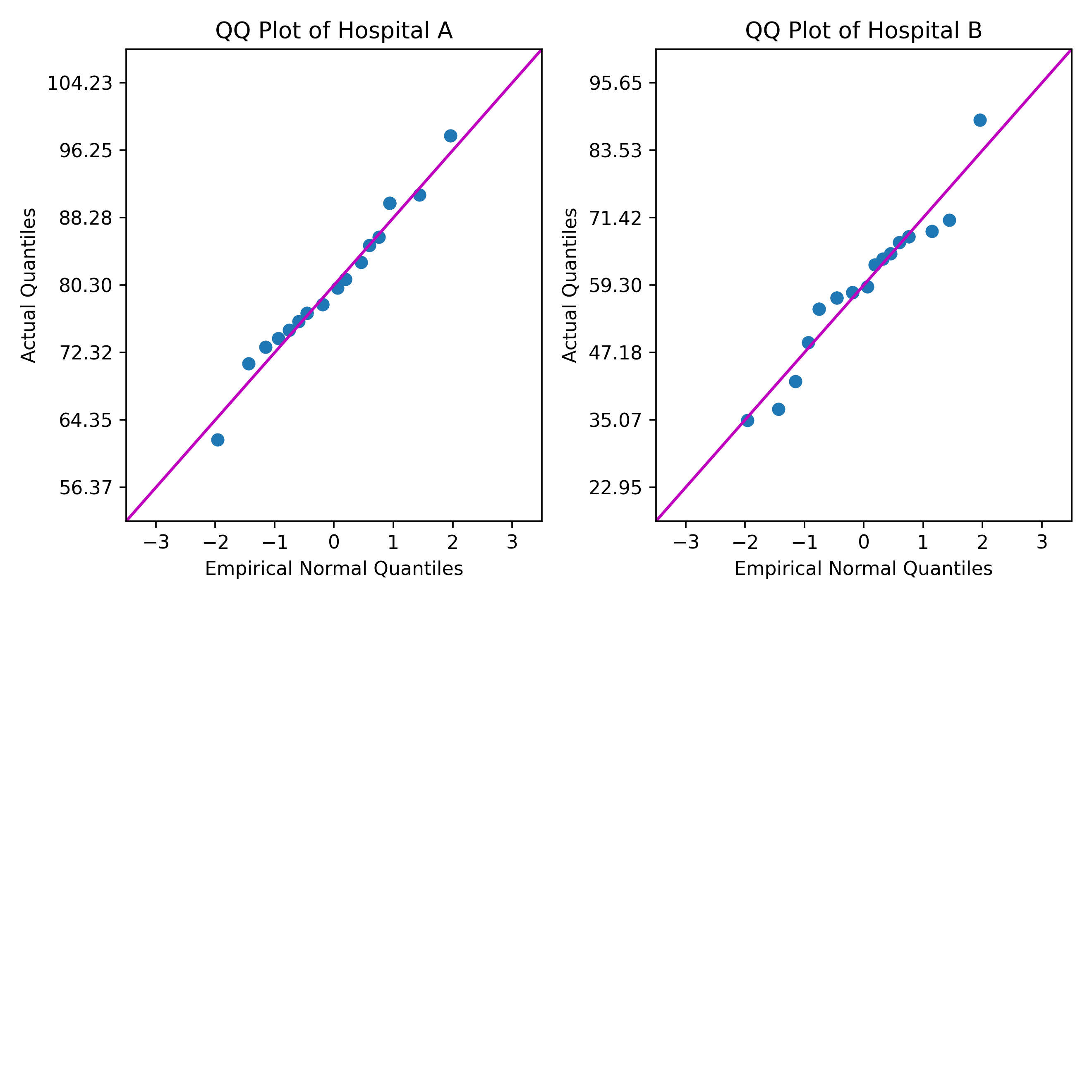
一位医疗保健顾问希望使用分位数-分位数 (QQ) 图比较两家医院患者满意度评级的正态性。QQ 图显示了每组患者满意度评级对正态分布的拟合优度。
Python 脚本示例从 Minitab 中的列读取数据。该脚本计算分位数,并为每列创建一个 QQ 图。然后,脚本将图发送到 Minitab“输出”窗格。
以下 .ZIP 文件提供了本指南中引用的所有文件:python_guide_files.zip。
使用以下文件执行本节中的步骤:
| 文件 | 说明 |
|---|---|
| qq_plot.py | Python 脚本,用于从 Minitab 工作表中获取列并显示每个列的 QQ 图。 |
以下示例中的 Python 脚本需要以下 Python 模块:括号中的数字是我们用于运行脚本的最新包版本。
- mtbpy
- 集成 Minitab 与 Python 的 Python 模块。在该示例中,此模块中的函数将 Python 结果发送到 Minitab。
- numpy (1.24.2)
- 具有各种科学和数字计算应用的 Python 模块。
- matplotlib (3.7.0)
- Python 模块,其具有与绘制图形和创建图表相关的各种功能。
- 确保已安装所需模块:mtbpy 和 numpy。
- 要通过 PIP 安装所需模块,请为操作系统的终端(例如,Microsoft® Windows Command Prompt或 macOS 终端)运行相应的命令:
pip install mtbpy numpy matplotlib
- 要通过 PIP 安装所需模块,请为操作系统的终端(例如,Microsoft® Windows Command Prompt或 macOS 终端)运行相应的命令:
- 将 Python 脚本文件 qq_plot.py 保存到 Minitab 默认文件位置。 有关 Minitab 在何处查找 Python 脚本文件的更多信息,可转到 Minitab 的 Python 文件的默认文件夹。
- 打开样本数据集酒店比较未堆叠.MWX。
-
在 Minitab 命令行窗格中,输入
PYSC "qq_plot.py" "Hospital A" "Hospital B"。 - 单击 运行。
qq_plot.py
"""
Description:
_________________________________________________________________________________
This script will generate a QQ Plot for each column of data passed to PYSC.
If PYSC was not given any columns, the script will look for data in every
column starting with the first column (C1) and ending at the first empty column.
The ranks are calculated using the Modified Kaplan-Meier method,
and duplicate values are given the same rank and quantile, this is also known
as "competition" ranking.
_________________________________________________________________________________
Imports:
_________________________________________________________________________________
numbers - For testing the types of the values in the data columns.
sys - For retrieving any columns passed from Minitab.
statistics - For calculating the inverse CDF of the normal distribution.
numpy - For general calculations and manipulating data.
matplotlib - For creating the plots.
mtbpy - For sending and receiving data with Minitab.
_________________________________________________________________________________
"""
import numbers
import sys
from statistics import NormalDist

import numpy as np
from matplotlib import pyplot as plt
from mtbpy import mtbpy

# sys.argv contains the arguments passed to PYSC, with sys.argv[0] being the name of the Python script file,
# and sys.argv[1:] being the list of columns passed after the name of Python script file,
# sys.argv[1:] has a length of 0 if no columns are passed to the PYSC command.
column_names = sys.argv[1:]

# If column_names is empty, loop over each column, starting at C1, and check if they contain data.
# Stop at the first column that does not contain data, and use the range of columns before that column.
if len(column_names) == 0:
    i = 1
    while mtbpy.mtb_instance().get_column(f"C{i}") is not None:
        column_names.append(f"C{i}")
        i += 1

# If there are no columns to analyze, throw an error stating that columns need to be passed or the data needs to start in C1
if len(column_names) == 0 or mtbpy.mtb_instance().get_column(column_names[0]) is None:
    raise IndexError("Worksheet is empty or column data could not be found!\n\tPass columns to PYSC or move first column to C1.")

# Initialize a list to store data from columns in a list of lists.
columns_data = []
# Loop through each column name.
for column_name in column_names:
    # Use mtbpy to get the data from Minitab for the column as a Python list.
    column_data = mtbpy.mtb_instance().get_column(column_name)
    # If any value in the data is not numeric, throw an error stating that only numeric columns can be used.
    if not all(isinstance(value, numbers.Number) for value in column_data):
        raise ValueError("Data is not numeric!\n\tPass only numeric columns to PYSC or delete non-numeric columns.")
    # Sort the data for calculation of quantiles.
    sorted_column_data = np.sort(column_data)
    # Append the sorted data to our list of column data.
    columns_data.append(sorted_column_data)

# Initialize a figure with:
# Figure Columns = 2 plus the number of data columns modulo 2.
# Figure Rows = Number of data columns floor-divided by the number of figure columns plus 1.
num_plot_cols = 2 + len(columns_data) % 2
num_plot_rows = len(columns_data) // num_plot_cols + 1
fig = plt.figure(figsize=(num_plot_cols * 4, num_plot_rows * 4), tight_layout=True)

# Iterate over the columns and generate a QQ Plot for each column.
for index, column_data in enumerate(columns_data):
    # Create an axis on the figure.
    current_axis = fig.add_subplot(num_plot_rows, num_plot_cols, index + 1)
    # Calculate the quantile of each data point in the column.
    # This uses the Modified Kaplan-Meier ranks, however, the ranks produced by
    # the numpy.searchsorted method begin at "0" and not "1," which would result
    # in negative rank values when using the Modified Kaplan-Meier method.
    # Therefore, the calculation uses rank + 1.0 - 0.5, which simplifies to rank + 0.5.
    column_ranks = np.searchsorted(np.sort(column_data), column_data) + 0.5
    # The quantiles are the ranks divided by the count.
    quantiles = column_ranks / len(column_data)

    # The tick marks on the y-axis and the fit line use the sample mean and sample standard deviation.
    column_mean = np.mean(column_data)
    column_stdev = np.std(column_data)

    # Calculate the empirical quantiles from the normal distribution.
    empirical_quantiles = [NormalDist().inv_cdf(x) for x in quantiles]

    # Create a scatterplot of the sample data versus the empirical quantiles.
    current_axis.scatter(empirical_quantiles, column_data)

    # Create a fit line for a perfect empirical normal distribution, for the scale of this plot, the fit line is 45 degrees.
    current_axis.plot([-3.5, 3.5], [column_mean-3.5*column_stdev, column_mean+3.5*column_stdev], "-m")

    # Set the title for the plot.
    current_axis.set_title(f"QQ Plot of {column_names[index]}")
    # Set the x axis label, bounds, and tick mark positions.
    current_axis.set_xlabel("Empirical Normal Quantiles")
    current_axis.set_xbound(lower=-3.5, upper=3.5)
    current_axis.set_xticks([-3, -2, -1, 0, 1, 2, 3])
    # Set the y axis label, bounds, and tick mark positions.
    current_axis.set_ylabel("Actual Quantiles")
    current_axis.set_ybound(lower=column_mean-3.5*column_stdev,
                            upper=column_mean+3.5*column_stdev)
    current_axis.set_yticks([column_mean-3*column_stdev,
                             column_mean-2*column_stdev,
                             column_mean-1*column_stdev,
                             column_mean,
                             column_mean+1*column_stdev,
                             column_mean+2*column_stdev,
                             column_mean+3*column_stdev])

# Save the combined plots figure as a PNG file.
fig.savefig("qqplot.png", dpi=330)

# Send the figure to Minitab.
mtbpy.mtb_instance().add_image("qqplot.png")
结果
Python Script