Note
This command is available with the Predictive Analytics Module. Click here for more information about how to activate the module.
Search for the best type of model
Researchers for a healthcare system collect data from their regional medical clinics. In particular, the research team is interested in data from doctors' initial examinations of sick patients. At the end of the initial examinations, the doctors assign each patient a score for the severity of their illness. The researchers want to develop a short questionnaire to help prioritize the sickest patients before examination by a doctor. Through consultation with subject matter experts and initial exploration of the data, the team selects 8 variables to predict the severity score. The researchers want to determine the best type of model to predict the severity score before they further refine the model.
The researchers use Discover Best Model (Continuous Response) to compare the predictive performance of 5 types of models: multiple regression, TreeNet®, Random Forests® CART® and MARS®. The team plans to further explore the type of model with the best predictive performance.
- Open the sample data, Illness.mtw.
- Choose .
- In Response, enter 'Illness Severity Score'.
- In Continuous predictors, enter 'Number of Symptoms Now'.
- In Categorical predictors, enter 'High Production of Phlegm'-'Limits on Normal Activities'.
- Click OK.
Interpret the results
The Model Selection table compares the performance of the types of models. The multiple regression model has the maximum value of R2. The results that follow are for the best multiple regression model.
To determine whether the association between the response and each term in the model is statistically significant, compare the p-value for the term to your significance level to assess the null hypothesis. The null hypothesis is that there is no association between the term and the response. Usually, a significance level (denoted as α or alpha) of 0.05 works well. A significance level of 0.05 indicates a 5% risk of concluding that an association exists when there is no actual association. In these results, two of the interaction terms have p-values that are greater than 0.05: Severe Shortness of Breath*Severe Headache and Severe Headache*Severe Sleep Disturbance. When the researchers explore other multiple regression models, they will use model performance metrics and residual plots to explore the effects of including these terms in the model.
The Model summary table shows that the training R2 and the test R2 are both approximately 91%. The test root mean squared error (RMSE), which represents how far the data values fall from the fitted values, is approximately 4. Because the RMSE is small on the scale of the illness score, the researchers are optimistic that a small number of questions is enough information to help prioritize patients.
The table of fits and diagnostics for unusual information shows data points that do not follow the proposed regression equation well. These are the fits and diagnostics from the full data set.
The letter R indicates a point with a large residual. Examine the unusual data points to see predictor values where the model might not fit well. The letter X indicates a point with high leverage. Points with high leverage have unusual predictor combinations relative to the rest of the data set.
Large residuals and high leverage points are potentially influential points. For example, the inclusion or exclusion of an influential point can change whether a coefficient is statistically significant or not. If you see an influential observation, determine whether the observation is a data-entry or measurement error. If the observation is not an error, determine how much the observation influences the results. When the researchers further explore the model, they will fit the model with and without the observations. Then, they will compare the coefficients, p-values, R2, and other model information. If the model changes significantly when you remove the influential observation, examine the model further to determine if you have incorrectly specified the model. You may need to gather more data to resolve the issue.
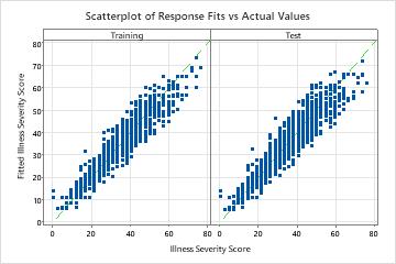
The scatterplot of the fitted illness scores versus actual illness scores shows the relationship between the fitted and actual values for both the training and test data. The points fall approximately near the reference line of y=x, which indicates that the model fits the data well.
Method
| Fit a regression model with linear terms and terms of order 2. |
|---|
| Fit 6 TreeNet® Regression model(s) using squared loss function. |
| Fit 3 Random Forests® Regression model(s) with bootstrap sample size same as training data size of 1546. |
| Fit an optimal CART® Regression model. |
| Fit an optimal MARS® Regression model. |
| Select the model with maximum R-squared from 5-fold cross-valuation. |
| Total number of rows: 1546 |
| Rows used for regression model: 1546 |
| Rows used for tree-based models: 1546 |
Response Information
| Mean | StDev | Minimum | Q1 | Median | Q3 | Maximum |
|---|---|---|---|---|---|---|
| 31.0110 | 14.0820 | 0 | 19.05 | 30.95 | 40.48 | 76.19 |
| Best Model within Type | R-squared (%) | Mean Absolute Deviation |
|---|---|---|
| Multiple Regression* | 91.23 | 3.1011 |
| MARS® | 91.05 | 3.1604 |
| TreeNet® | 90.90 | 3.1613 |
| Random Forests® | 89.93 | 3.3248 |
| CART® | 86.11 | 3.9369 |
Forward Selection of Terms with Validation for Best Multiple Regression Model
Breath, Severe Headache, Severe Sleep Disturbance, Generally Feeling Very Bad, Limits on
Normal Activities, Number of Symptoms Now*Severe Shortness of Breath, Number of Symptoms
Now*Severe Chest Pain, Severe Shortness of Breath*Severe Sleep Disturbance, Generally Feeling
Very Bad*Limits on Normal Activities
Regression Equation
| Illness Severity Score | = | 1.241 + 2.5386 Number of Symptoms Now + 0.0 High Production of Phlegm_0 + 3.900 High Production of Phlegm_1 + 0.0 Severe Shortness of Breath_0 + 0.94 Severe Shortness of Breath_1 + 0.0 Severe Headache_0 + 4.094 Severe Headache_1 + 0.0 Severe Sleep Disturbance_0 + 3.884 Severe Sleep Disturbance_1 + 0.0 Generally Feeling Very Bad_0 + 3.473 Generally Feeling Very Bad_1 + 0.0 Limits on Normal Activities_0 + 3.140 Limits on Normal Activities_1 + 0.0 Number of Symptoms Now*Severe Shortness of Breath_0 + 0.373 Number of Symptoms Now*Severe Shortness of Breath_1 + 0.0 Number of Symptoms Now*Severe Chest Pain_0 + 0.4765 Number of Symptoms Now*Severe Chest Pain_1 + 0.0 Severe Shortness of Breath*Severe Sleep Disturbance_0 0 + 0.0 Severe Shortness of Breath*Severe Sleep Disturbance_0 1 + 0.0 Severe Shortness of Breath*Severe Sleep Disturbance_1 0 + 1.337 Severe Shortness of Breath*Severe Sleep Disturbance_1 1 + 0.0 Generally Feeling Very Bad*Limits on Normal Activities_0 0 + 0.0 Generally Feeling Very Bad*Limits on Normal Activities_0 1 + 0.0 Generally Feeling Very Bad*Limits on Normal Activities_1 0 + 1.372 Generally Feeling Very Bad*Limits on Normal Activities_1 1 |
|---|
Coefficients
| Term | Coef | SE Coef | T-Value | P-Value |
|---|---|---|---|---|
| Constant | 1.241 | 0.385 | 3.22 | 0.001 |
| Number of Symptoms Now | 2.5386 | 0.0593 | 42.81 | 0.000 |
| High Production of Phlegm | ||||
| 1 | 3.900 | 0.225 | 17.35 | 0.000 |
| Severe Shortness of Breath | ||||
| 1 | 0.94 | 1.18 | 0.80 | 0.424 |
| Severe Headache | ||||
| 1 | 4.094 | 0.253 | 16.18 | 0.000 |
| Severe Sleep Disturbance | ||||
| 1 | 3.884 | 0.284 | 13.69 | 0.000 |
| Generally Feeling Very Bad | ||||
| 1 | 3.473 | 0.343 | 10.14 | 0.000 |
| Limits on Normal Activities | ||||
| 1 | 3.140 | 0.424 | 7.40 | 0.000 |
| Number of Symptoms Now*Severe Shortness of Breath | ||||
| 1 | 0.373 | 0.133 | 2.81 | 0.005 |
| Number of Symptoms Now*Severe Chest Pain | ||||
| 1 | 0.4765 | 0.0312 | 15.26 | 0.000 |
| Severe Shortness of Breath*Severe Sleep Disturbance | ||||
| 1 1 | 1.337 | 0.528 | 2.53 | 0.011 |
| Generally Feeling Very Bad*Limits on Normal Activities | ||||
| 1 1 | 1.372 | 0.527 | 2.61 | 0.009 |
| Term | VIF |
|---|---|
| Constant | |
| Number of Symptoms Now | 1.95 |
| High Production of Phlegm | |
| 1 | 1.10 |
| Severe Shortness of Breath | |
| 1 | 23.23 |
| Severe Headache | |
| 1 | 1.25 |
| Severe Sleep Disturbance | |
| 1 | 1.73 |
| Generally Feeling Very Bad | |
| 1 | 2.62 |
| Limits on Normal Activities | |
| 1 | 3.98 |
| Number of Symptoms Now*Severe Shortness of Breath | |
| 1 | 26.80 |
| Number of Symptoms Now*Severe Chest Pain | |
| 1 | 1.25 |
| Severe Shortness of Breath*Severe Sleep Disturbance | |
| 1 1 | 3.26 |
| Generally Feeling Very Bad*Limits on Normal Activities | |
| 1 1 | 5.73 |
Model Summary
| Statistics | Training | Test |
|---|---|---|
| R-squared | 91.35% | 91.23% |
| Root mean squared error (RMSE) | 4.1562 | 4.1679 |
| Mean squared error (MSE) | 17.2741 | 17.3714 |
| Mean absolute deviation (MAD) | 3.0798 | 3.1011 |
| R-squared (adj) | 91.29% | |
| R-squared (pred) | 91.19% |
Analysis of Variance
| Source | DF | Adj SS | Adj MS | F-Value |
|---|---|---|---|---|
| Regression | 11 | 279881 | 25443.7 | 1472.94 |
| Number of Symptoms Now | 1 | 31655 | 31654.8 | 1832.51 |
| High Production of Phlegm | 1 | 5202 | 5201.8 | 301.14 |
| Severe Shortness of Breath | 1 | 11 | 11.1 | 0.64 |
| Severe Headache | 1 | 4520 | 4520.0 | 261.66 |
| Severe Sleep Disturbance | 1 | 3239 | 3238.8 | 187.50 |
| Generally Feeling Very Bad | 1 | 1776 | 1775.6 | 102.79 |
| Limits on Normal Activities | 1 | 945 | 945.4 | 54.73 |
| Number of Symptoms Now*Severe Shortness of Breath | 1 | 136 | 136.4 | 7.90 |
| Number of Symptoms Now*Severe Chest Pain | 1 | 4023 | 4023.4 | 232.92 |
| Severe Shortness of Breath*Severe Sleep Disturbance | 1 | 111 | 110.7 | 6.41 |
| Generally Feeling Very Bad*Limits on Normal Activities | 1 | 117 | 117.3 | 6.79 |
| Error | 1534 | 26498 | 17.3 | |
| Lack-of-Fit | 484 | 9247 | 19.1 | 1.16 |
| Pure Error | 1050 | 17251 | 16.4 | |
| Total | 1545 | 306379 |
| Source | P-Value |
|---|---|
| Regression | 0.000 |
| Number of Symptoms Now | 0.000 |
| High Production of Phlegm | 0.000 |
| Severe Shortness of Breath | 0.424 |
| Severe Headache | 0.000 |
| Severe Sleep Disturbance | 0.000 |
| Generally Feeling Very Bad | 0.000 |
| Limits on Normal Activities | 0.000 |
| Number of Symptoms Now*Severe Shortness of Breath | 0.005 |
| Number of Symptoms Now*Severe Chest Pain | 0.000 |
| Severe Shortness of Breath*Severe Sleep Disturbance | 0.011 |
| Generally Feeling Very Bad*Limits on Normal Activities | 0.009 |
| Error | |
| Lack-of-Fit | 0.025 |
| Pure Error | |
| Total |
Fits and Diagnostics for Unusual Observations
| Obs | Illness Severity Score | Fit | Resid | Std Resid | ||
|---|---|---|---|---|---|---|
| 11 | 66.670 | 56.757 | 9.913 | 2.40 | R | |
| 13 | 52.380 | 41.177 | 11.203 | 2.71 | R | |
| 16 | 59.520 | 48.604 | 10.916 | 2.64 | R | |
| 33 | 50.000 | 60.657 | -10.657 | -2.57 | R | |
| 48 | 64.290 | 55.416 | 8.874 | 2.14 | R | |
| 52 | 61.900 | 53.369 | 8.531 | 2.06 | R | |
| 54 | 50.000 | 41.598 | 8.402 | 2.03 | R | |
| 56 | 50.000 | 58.328 | -8.328 | -2.02 | R | |
| 58 | 38.100 | 46.485 | -8.385 | -2.03 | R | |
| 106 | 59.520 | 49.028 | 10.492 | 2.53 | R | |
| 114 | 59.520 | 47.160 | 12.360 | 2.99 | R | |
| 128 | 69.050 | 58.328 | 10.722 | 2.59 | R | |
| 144 | 50.000 | 40.471 | 9.529 | 2.30 | R | |
| 173 | 47.620 | 56.757 | -9.137 | -2.21 | R | |
| 174 | 42.860 | 34.000 | 8.860 | 2.14 | R | |
| 191 | 42.860 | 52.051 | -9.191 | -2.23 | R | |
| 198 | 59.520 | 48.411 | 11.109 | 2.68 | R | |
| 202 | 73.810 | 64.046 | 9.764 | 2.36 | R | |
| 205 | 47.620 | 37.559 | 10.061 | 2.43 | R | |
| 213 | 35.710 | 34.970 | 0.740 | 0.18 | X | |
| 217 | 16.670 | 19.053 | -2.383 | -0.58 | X | |
| 239 | 47.620 | 58.328 | -10.708 | -2.59 | R | |
| 241 | 71.430 | 66.311 | 5.119 | 1.25 | X | |
| 243 | 14.290 | 24.088 | -9.798 | -2.36 | R | |
| 304 | 50.000 | 41.130 | 8.870 | 2.14 | R | |
| 307 | 14.290 | 10.920 | 3.370 | 0.83 | X | |
| 352 | 64.290 | 51.254 | 13.036 | 3.15 | R | |
| 369 | 38.100 | 49.275 | -11.175 | -2.70 | R | |
| 391 | 16.670 | 32.073 | -15.403 | -3.72 | R | |
| 392 | 0.000 | 11.395 | -11.395 | -2.75 | R | |
| 395 | 0.000 | 13.934 | -13.934 | -3.36 | R | |
| 424 | 40.480 | 52.504 | -12.024 | -2.90 | R | |
| 425 | 47.620 | 34.597 | 13.023 | 3.16 | R | |
| 474 | 47.620 | 38.538 | 9.082 | 2.21 | R | |
| 479 | 40.480 | 30.896 | 9.584 | 2.31 | R | |
| 489 | 16.670 | 25.023 | -8.353 | -2.02 | R | |
| 491 | 30.950 | 24.348 | 6.602 | 1.61 | X | |
| 493 | 57.140 | 44.339 | 12.801 | 3.09 | R | |
| 495 | 35.710 | 25.480 | 10.230 | 2.47 | R | |
| 509 | 38.100 | 26.696 | 11.404 | 2.77 | R | |
| 520 | 73.810 | 58.328 | 15.482 | 3.75 | R | |
| 537 | 38.100 | 28.358 | 9.742 | 2.35 | R | |
| 550 | 14.290 | 24.458 | -10.168 | -2.45 | R | |
| 583 | 42.860 | 53.369 | -10.509 | -2.54 | R | |
| 694 | 19.050 | 21.817 | -2.767 | -0.68 | X | |
| 720 | 59.520 | 65.602 | -6.082 | -1.49 | X | |
| 722 | 40.480 | 32.066 | 8.414 | 2.03 | R | |
| 802 | 30.950 | 42.586 | -11.636 | -2.81 | R | |
| 805 | 30.950 | 39.868 | -8.918 | -2.16 | R | |
| 814 | 40.480 | 32.073 | 8.407 | 2.03 | R | |
| 823 | 61.900 | 48.148 | 13.752 | 3.33 | R | |
| 833 | 33.330 | 44.054 | -10.724 | -2.60 | R | |
| 859 | 38.100 | 49.275 | -11.175 | -2.70 | R | |
| 868 | 47.620 | 37.789 | 9.831 | 2.38 | R | |
| 891 | 30.950 | 19.945 | 11.005 | 2.66 | R | |
| 893 | 28.570 | 48.860 | -20.290 | -4.92 | R | |
| 905 | 45.240 | 55.416 | -10.176 | -2.46 | R | |
| 924 | 54.760 | 56.019 | -1.259 | -0.31 | X | |
| 977 | 64.290 | 53.107 | 11.183 | 2.72 | R | |
| 983 | 57.140 | 47.683 | 9.457 | 2.29 | R | |
| 988 | 50.000 | 44.501 | 5.499 | 1.34 | X | |
| 993 | 73.810 | 64.046 | 9.764 | 2.36 | R | |
| 997 | 33.330 | 24.458 | 8.872 | 2.14 | R | |
| 1003 | 54.760 | 45.128 | 9.632 | 2.33 | R | |
| 1025 | 33.330 | 47.705 | -14.375 | -3.49 | R | |
| 1059 | 57.140 | 48.663 | 8.477 | 2.05 | R | |
| 1105 | 47.620 | 37.319 | 10.301 | 2.49 | R | |
| 1150 | 59.520 | 44.339 | 15.181 | 3.67 | R | |
| 1160 | 52.380 | 40.051 | 12.329 | 2.97 | R | |
| 1163 | 30.950 | 41.598 | -10.648 | -2.57 | R | |
| 1165 | 69.050 | 56.757 | 12.293 | 2.97 | R | |
| 1169 | 59.520 | 49.275 | 10.245 | 2.48 | R | |
| 1198 | 42.860 | 51.516 | -8.656 | -2.09 | R | |
| 1207 | 76.190 | 63.534 | 12.656 | 3.07 | R | |
| 1213 | 26.190 | 40.278 | -14.088 | -3.41 | R | |
| 1228 | 40.480 | 50.571 | -10.091 | -2.45 | R | |
| 1235 | 59.520 | 50.175 | 9.345 | 2.26 | R | |
| 1237 | 57.140 | 48.239 | 8.901 | 2.15 | R | |
| 1246 | 64.290 | 55.416 | 8.874 | 2.14 | R | |
| 1262 | 45.240 | 35.957 | 9.283 | 2.24 | R | |
| 1263 | 57.140 | 43.951 | 13.189 | 3.18 | R | |
| 1282 | 33.330 | 36.011 | -2.681 | -0.65 | X | |
| 1284 | 45.240 | 56.564 | -11.324 | -2.74 | R | |
| 1285 | 47.620 | 60.657 | -13.037 | -3.15 | R | |
| 1303 | 26.190 | 36.567 | -10.377 | -2.51 | R | |
| 1305 | 35.710 | 45.499 | -9.789 | -2.36 | R | |
| 1311 | 30.950 | 40.089 | -9.139 | -2.21 | R | |
| 1345 | 26.190 | 25.105 | 1.085 | 0.26 | X | |
| 1353 | 42.860 | 53.175 | -10.315 | -2.49 | R | |
| 1365 | 26.190 | 17.834 | 8.356 | 2.01 | R | |
| 1377 | 47.620 | 35.222 | 12.398 | 3.00 | R | |
| 1380 | 69.050 | 55.416 | 13.634 | 3.29 | R | |
| 1384 | 50.000 | 38.496 | 11.504 | 2.78 | R | |
| 1414 | 26.190 | 35.345 | -9.155 | -2.21 | R | |
| 1502 | 61.900 | 50.195 | 11.705 | 2.84 | R | |
| 1526 | 38.100 | 25.450 | 12.650 | 3.05 | R | |
| 1535 | 14.290 | 24.088 | -9.798 | -2.36 | R | |
| 1544 | 38.100 | 29.165 | 8.935 | 2.16 | R | |
| 1548 | 50.000 | 40.455 | 9.545 | 2.31 | R | |
| 1565 | 38.100 | 42.846 | -4.746 | -1.16 | X | |
| 1582 | 66.670 | 55.437 | 11.233 | 2.72 | R |
Select an alternative model
The researchers decide to examine the results for the best TreeNet® model.
- In the results for Discover Best Model (Continuous Response), after the Stepwise Selection of Terms for Best Multiple Regression Model, click Select an Alternative Model.
- In Model Type, select TreeNet®.
- In Select an existing model, choose the sixth model, which has the best value of R2.
- Click Display Results.
Interpret the results
This analysis grows 300 trees and the optimal number of trees is 63. The model uses a learning rate of 0.1 and a subsample fraction of 0.7. The maximum number of terminal nodes is 6.
Method
| Loss function | Squared error |
|---|---|
| Criterion for selecting optimal number of trees | Maximum R-squared |
| Model validation | 5-fold cross-validation |
| Learning rate | 0.1 |
| Subsample fraction | 0.7 |
| Maximum terminal nodes per tree | 6 |
| Minimum terminal node size | 3 |
| Number of predictors selected for node splitting | Total number of predictors = 8 |
| Rows used | 1546 |
| Rows unused | 70 |
Response Information
| Mean | StDev | Minimum | Q1 | Median | Q3 | Maximum |
|---|---|---|---|---|---|---|
| 31.0110 | 14.0820 | 0 | 19.05 | 30.95 | 40.48 | 76.19 |
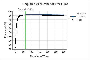
The R-squared vs Number of Trees Plot shows the entire curve over the number of trees grown. The optimal value for the test data is about 91% when the number of trees is 63.
Model Summary
| Total predictors | 8 |
|---|---|
| Important predictors | 8 |
| Number of trees grown | 300 |
| Optimal number of trees | 63 |
| Statistics | Training | Test |
|---|---|---|
| R-squared | 91.93% | 90.90% |
| Root mean squared error (RMSE) | 3.9992 | 4.2471 |
| Mean squared error (MSE) | 15.9932 | 18.0375 |
| Mean absolute deviation (MAD) | 2.9943 | 3.1613 |
| Mean absolute percent error (MAPE) | 0.1088 | 0.1130 |
The Model summary table shows that the R2 value when the number of trees is 63 is approximately 92% for the training data and approximately 91% for the test data.
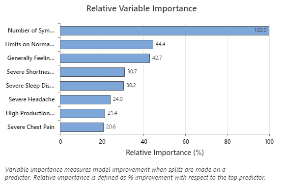
The Relative Variable Importance graph plots the predictors in order of their effect on model improvement when splits are made on a predictor over the sequence of trees. The most important predictor variable is Number of Symptoms Now. If the contribution of the top predictor variable, Number of Symptoms Now, is 100%, then the next important variable, Limits on Normal Activities, has a contribution of 44.4%. This means Limits on Normal Activities is 44.4% as important as Number of Symptoms Now in this regression model.
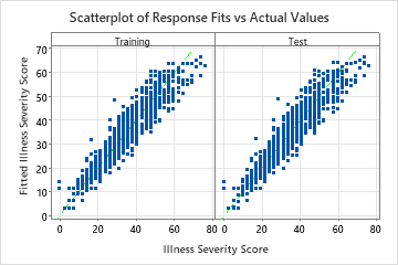
The scatterplot of the fitted illness scores versus actual illness scores shows the relationship between the fitted and actual values for both the training and test data. The points fall approximately near the reference line of y=x, which indicates that the model fits the data well.
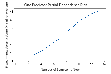
Use the partial dependency plots to gain insight into how the important variables or pairs of variables affect the fitted response values. The partial dependence plots show whether the relationship between the response and a variable is linear, monotonic, or more complex.
The first plot illustrates the relationship between the illness scores and the number of symptoms the patient has now. You can hover over individual data points to see the specific x- and y-values. For instance, the highest point on the right side of the graph is when the patient has 13 symptoms and the fitted illness score is approximately 45.
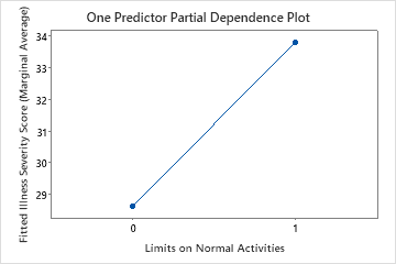
The second plot illustrates that the fitted illness score increases by approximately 5 points when patients report limitations on their normal activities.
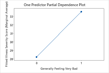
The third plot illustrates that the fitted illness score increases by approximately 5 points when patients report generally feeling very bad.
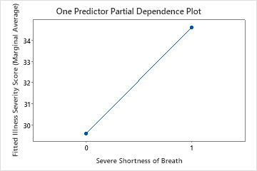
The fourth plot illustrates the fitted illness score increases by approximately 4 points when patients report severe shortness of breath.
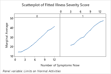
The last plot illustrates how the fitted illness score for a number of symptoms depends on whether the patient also has limits on their normal activities. For the same number of symptoms, patients who also report limits on their normal activities have higher fitted illness scores.