Methods and formulas for the analysis of variance in Analyze Factorial Design

In This Topic

Sum of squares (SS)
Sequential sum of squares
Adjusted sum of squares
Degrees of freedom (DF)
Adj MS – Term

F
P-value – Analysis of variance table
Pure error lack-of-fit test
P-value – Lack-of-fit test

Sum of squares (SS)

The sum of squared distances. The formulas presented are for a full factorial, two-factor model with factors A and B. These formulas can be extended to models with more than two factors. For information, see Montgomery¹.

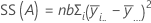
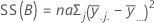
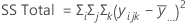
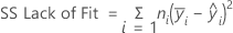
SS Total is the total variation in the model. SS (A) and SS (B) are the sum of the squared deviations of the estimated factor level means around the overall mean. SS Error is the sum of the squared residuals. It is also known as error within treatments. The calculations are:

If the model includes replicates, SS Pure Error is:

For different cases than the full factorial, two-factor model, you can have other sums of squares. If you fit a reduced model, SS Lack of Fit is:

If the model includes center points, SS Curvature is:

In split-plot designs, the sums of squares for whole plot and subplot error variation are:

D.C. Montgomery (1991). Design and Analysis of Experiments, Third Edition, John Wiley & Sons.

Notation

Term	Description
a	number of levels in factor A
b	number of levels in factor B
n	total number of replicates
	mean of the i^th level of factor A
	overall mean of all observations
	mean of the j^th level of factor B
	observation at the i^th level of factor A, j^th level of factor B, and the k^th replicate
	mean of the i^th level of factor A and j^th level of factor B
	mean response for center points
	mean response for factorial points
n_F	number of factorial points

Sequential sum of squares

Minitab breaks down the SS Regression or Treatments component of variance into sequential sums of squares for each factor. The sequential sums of squares depend on the order the factors or predictors are entered into the model. The sequential sum of squares is the unique portion of SS Regression explained by a factor, given any previously entered factors.

For example, if you have a model with three factors or predictors, X1, X2, and X3, the sequential sum of squares for X2 shows how much of the remaining variation X2 explains, given that X1 is already in the model. To obtain a different sequence of factors, repeat the analysis and enter the factors in a different order.

Adjusted sum of squares

The adjusted sums of squares does not depend on the order that the terms enter the model. The adjusted sum of squares is the amount of variation explained by a term, given all other terms in the model, regardless of the order that the terms enter the model.

For example, if you have a model with three factors, X1, X2, and X3, the adjusted sum of squares for X2 shows how much of the remaining variation the term for X2 explains, given that the terms for X1 and X3 are also in the model.

The calculations for the adjusted sums of squares for three factors are:

SSR(X3 | X1, X2) = SSE (X1, X2) - SSE (X1, X2, X3) or
SSR(X3 | X1, X2) = SSR (X1, X2, X3) - SSR (X1, X2)

where SSR(X3 | X1, X2) is the adjusted sum of squares for X3, given that X1 and X2 are in the model.

SSR(X2, X3 | X1) = SSE (X1) - SSE (X1, X2, X3) or
SSR(X2, X3 | X1) = SSR (X1, X2, X3) - SSR (X1)

where SSR(X2, X3 | X1) is the adjusted sum of squares for X2 and X3, given that X1 is in the model.

You can extend these formulas if you have more than 3 factors in your model¹.

J. Neter, W. Wasserman and M.H. Kutner (1985). Applied Linear Statistical Models, Second Edition. Irwin, Inc.

Degrees of freedom (DF)

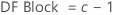
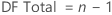
For a full factorial design with factors A and B, and a blocking variable, the number of degrees of freedom associated with each sum of squares is:

For interactions among factors, multiply the degrees of freedom for the terms in the factor. For example, if the factors are A and B then the interaction AB has these degrees of freedom:

To find the degrees of freedom for a type of term, sum the degrees of freedom for the terms. For example, if the factors are A and B then the main effects in the model have this many degrees of freedom:

For 2-level designs with center points, the degrees of freedom for curvature are 1.

Notation

Term	Description
a	number of levels in factor A
b	number of levels in factor B
c	number of blocks
n	total number of observations
n_i	number of observations for i^th factor level combination
m	number of factor level combinations
p	number of coefficients

Adj MS – Term

The calculation for the Mean Square (MS) for the model term is:

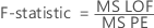
F

A test to determine whether the interaction and main effects are significant. The formula for the model terms is:

The degrees of freedom for the test are:

Numerator = degrees of freedom for term
Denominator = degrees of freedom for error

Larger values of F support rejecting the null hypothesis that there is not a significant effect.

For balanced split-plot designs, the F statistic for hard-to-change factors uses the MS for whole plot error in the denominator. For other split-plot designs, Minitab uses a linear combination of the WP Error and the SP Error to construct a denominator that is based on the expected mean squares.

P-value – Analysis of variance table

The p-value is a probability that is calculated from an F-distribution with the degrees of freedom (DF) as follows:

Numerator DF: sum of the degrees of freedom for the term or the terms in the test
Denominator DF: degrees of freedom for error

Formula

1 − P(F ≤ f_j)

Notation

Term	Description
P(F ≤ f)	cumulative distribution function for the F-distribution
f	f-statistic for the test

Pure error lack-of-fit test

To calculate the pure error lack-of-fit test, Minitab calculates:

The sum of squared deviations of the response from the mean within each set of replicates and adds them together to create the pure error sum of squares (SS PE).
The pure error mean square

where n = number of observations and m = number of distinct x-level combinations
The lack-of-fit sum of squares
The lack-of-fit mean square
The test statistics

Large F-values and small p-values suggest that the model is inadequate.

P-value – Lack-of-fit test

This p-value is for the test of the null hypothesis that the coefficients are 0 for any terms that are possible to estimate from these data that are not in the model. The p-value is the probability from an F distribution with degrees of freedom (DF) as follows:

Numerator DF: degrees of freedom for lack-of-fit
Denominator DF: degrees of freedom for pure error

Formula

1 − P(F ≤ f_j)

Notation

Term	Description
P(F ≤ f_j)	cumulative distribution function for the F-distribution
f_j	f-statistic for the test