Step 1: Examine the calculated values
Using the values of the two properties that you entered, Minitab calculates the difference, the sample size, or the power of the test.
- Difference (or ratio)
- If you enter the sample size and the power of the test, then Minitab calculates the difference (or ratio) that the test can accommodate at the specified power and sample size. For larger sample sizes, the difference (or ratio) can be closer to your equivalence limits. This value represents the difference (or ratio) between the mean of the test population and the mean of the reference population.
- Sample size
- If you enter a difference and a power value for the test, then Minitab calculates how large your sample must be. If you increase the sample size, the power of the test also increases. You want enough observations in your sample to achieve adequate power. But you don't want a sample size so large that you waste time and money on unnecessary sampling or detect unimportant differences to be statistically significant.
Note
Because sample sizes are whole numbers, the actual power of the test might be slightly greater than the power value that you specify.
- Power
- If you enter a sample size and a difference (or ratio), then Minitab calculates the power of the test. A power value of at least 0.9 is usually considered adequate. A power of 0.9 indicates that you have a 90% chance of demonstrating equivalence when the difference (or ratio) between the population means is actually within the equivalence limits. If an equivalence test has low power, you might fail to demonstrate equivalence even when the test mean and the reference mean are equivalent. Usually, when the sample size is smaller or the difference is closer to an equivalence limit, the test has less power to claim equivalence.
Note
The definitions and interpretation in this topic apply to a standard equivalence test that uses the default alternative hypothesis (Lower limit < test mean - reference mean < upper limit).
Method
| Power for difference: | Test mean - reference mean |
|---|---|
| Null hypothesis: | Difference ≤ -0.45 or Difference ≥ 0.45 |
| Alternative hypothesis: | -0.45 < Difference < 0.45 |
| α level: | 0.05 |
Results
| Difference | Sample Size | Power |
|---|---|---|
| 0.4 | 12 | 0.603466 |
Key Results: Difference, Sample size, Power
These results show that if the sample size is 12 in each sequence and the difference is 0.4, then the power of the test to demonstrate equivalence is approximately 0.6. Because the power of the test is not adequate to accommodate a difference of 0.4, you should increase the sample size, if possible. You can also use the power curve to determine at what difference value the test may achieve adequate power (0.9) for the specified sample size.
Step 2: Examine the power curve
Use the power curve to assess the appropriate sample size or power for your test.
The power curve represents every combination of power and difference (or ratio) for each sample size when the significance level and the standard deviation (or coefficient of variation) are held constant. Each symbol on the power curve represents a calculated value based on the values that you enter. For example, if you enter a sample size and a power value, Minitab calculates the corresponding difference (or ratio) and displays the calculated value on the graph.
Examine the values on the curve to determine the difference (or ratio) between the test mean and the reference mean that can be accommodated at a certain power value and sample size. A power value of 0.9 is usually considered adequate. However, some practitioners consider a power value of 0.8 to be adequate. If an equivalence test has low power, you might fail to demonstrate equivalence even when the population means are equivalent. If you increase the sample size, the power of the test also increases. You want enough observations in your sample to achieve adequate power. But you don't want a sample size so large that you waste time and money on unnecessary sampling or detect unimportant differences to be statistically significant. Usually, differences (or ratios) that are closer to the equivalence limits require more power to demonstrate equivalence.
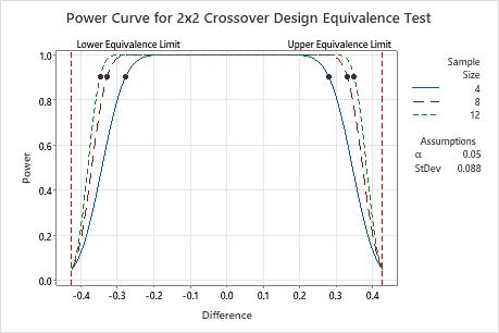
In this graph, the power curves for all sample sizes show that the test has adequate power (≥ 0.9) for a difference as large as approximately ±0.25. The sample sizes refer to the number of participants in each sequence. The power curve for a sample size of 4 shows that the test has a power of 0.9 for a difference of approximately ±0.28. The power curve for a sample size of 12 shows that the test has a power of 0.9 for a difference of approximately ±0.33. Notice that increasing the sample size to 12 only very slightly increases the difference that can be accommodated at a power of 0.9. For each curve, as the difference approaches the lower equivalence limit or the upper equivalence limit, the power of the test decreases and approaches α (alpha, which is the risk of claiming equivalence when it is not true).