Confidence interval (CI)
Formula
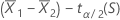 to
to 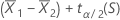
Notation
| Term | Description |
|---|---|
 | mean of the first sample |
 | mean of the second sample |
| tα/2 | inverse cumulative probability of a t distribution at 1 – α/2 |
| α | 1 - confidence level / 100 |
| s | sample standard deviation as calculated for the test statistic |
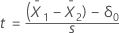
T-value
Formula
 depends upon the variance assumption.
- Unequal variances
-
When you assume unequal variances, the sample standard deviation of
 is:
is: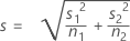
The degrees of freedom are:

If necessary, Minitab truncates the degrees of freedom to an integer, which is a more conservative approach than rounding.
- Equal variances
-
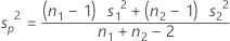
When you assume equal variances, the common variance is estimated by the pooled variance:
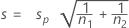
 The standard deviation of
 is estimated by:
The test statistic degrees of freedom are:
DF = n1 + n2 – 2
Notation
| Term | Description |
|---|---|
 | mean of the first sample |
 | mean of the second sample |
| s | sample standard deviation of  |
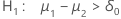
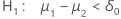
| δ0 | hypothesized difference between the two population means |
| s1 | sample standard deviation of the first sample |
| s2 | sample standard deviation of the second sample |
| n1 | sample size of the first sample |
| n2 | sample size of the second sample |
| VAR1 |  |
| VAR2 |  |
Calculate the pooled standard deviation
Suppose C1 contains the response, and C3 contains the mean for each factor level. For example:
| C1 | C2 | C3 |
|---|---|---|
| Response | Factor | Mean |
| 18.95 | 1 | 14.5033 |
| 12.62 | 1 | 14.5033 |
| 11.94 | 1 | 14.5033 |
| 14.42 | 2 | 10.5567 |
| 10.06 | 2 | 10.5567 |
| 7.19 | 2 | 10.5567 |
- Choose .
- In Store result in variable, enter C4.
- In Expression, enter SQRT((SUM((C1 - C3)**2)) / (total number of observations - number of groups)) . For the previous example, the Expression for the pooled standard deviation would be: SQRT((SUM(('Response' - 'Mean')**2)) / (6 - 2))
The value that Minitab stores is 3.75489.
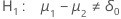
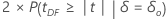
P-value
Formula
The calculation for the p-value depends on the alternative hypothesis.
| Alternative Hypothesis | P-value |
|---|---|
 |
 |
 |
 |
 |
 |
- Unequal variances
-
When you assume unequal variances, the degrees of freedom are:
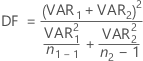
If necessary, Minitab truncates the degrees of freedom to an integer, which is a more conservative approach than rounding.
- Equal variances
-
When you assume equal variances, the test statistic degrees of freedom are:
DF = n1 + n2 – 2
Notation
| Term | Description |
|---|---|
| μ1 | population mean of the first sample |
| μ1 | population mean of the second sample |
| n1 | sample size of the first sample |
| n2 | sample size of the second sample |
| δ0 | hypothesized difference between the two population means |
| t | t-statistic from the sample data |
| t | a random variable from the t-distribution with DF degrees of freedom. |
| VAR1 |  |
| VAR2 |  |