엔진 공장의 품질 엔지니어가 두 공급업체의 피스톤에 대한 바이모달리티 테스트를 수행하려고 합니다. 엔지니어는 각 공급업체로부터 피스톤 100개를 랜덤 표본으로 추출하여 길이를 측정합니다.
스크립트는 R용 diptest 패키지를 사용하여 데이터가 단정상인지 여부를 테스트합니다. 검정이 단모달 데이터에 대한 귀무 가설을 기각하는 경우 스크립트는 데이터가 두 정규 분포의 혼합이라고 가정합니다. 스크립트는 R용 mixtools 패키지를 사용하여 두 정규 분포에 대한 기술 통계 및 밀도 곡선을 표시합니다.
예제 R 스크립트는 통합의 다음 기능을 보여줍니다.
- Minitab 워크시트의 단일 열을 입력으로 전달합니다.
- 표 제목을 추가합니다.
- 테이블에 대한 열 레이블을 추가합니다.
- Minitab 출력 창으로 표를 보냅니다.
- 그래프를 생성하고 그래프를 Minitab 출력 창으로 보냅니다.
다음 파일을 사용하여 이 섹션의 단계를 수행합니다.
| 파일 | 설명 |
|---|---|
| bimodal.R | R Minitab 워크시트에서 열을 가져와 단조성을 검정하고 데이터가 단형성이 아닌 경우 두 정규 분포의 혼합에 대한 결과를 생성하는 스크립트입니다. |
이 가이드에서 참조하는 모든 파일은 .ZIP 파일인 r_guide_files.zip.
사전 과정
-
아래 예제의 R 스크립트에는 다음 R 패키지가 필요합니다.
- mtbr
- Minitab과 R을 통합하는 R 패키지입니다. 예제에서는 이 모듈의 함수가 R 결과를 Minitab으로 보냅니다. Minitab 패키지를 설치하는 방법에 대한 자세한 내용은 2단계를 참조하십시오. R mtbr을 설치합니다.
- mixtools
- R 스크립트가 정규 분포의 혼합에 대한 출력을 만드는 데 사용하는 패키지입니다.
- diptest
- R 스크립트가 데이터가 단순 모드인지 여부를 테스트하는 데 사용하는 패키지입니다.
install.packages("mixtools")패키지 설치 R 에 대한 지원이 필요한 경우 조직의 기술 지원 부서에 문의하십시오. Minitab 기술 지원은 패키지 설치 R 를 지원할 수 없습니다.
예제를 실행하는 단계
- 필요한 모듈인 mtbr.
- R 스크립트 파일 bimodal.R를 Minitab 기본 파일 위치에 저장합니다. Minitab이 R 스크립트 파일을 찾는 위치에 대한 자세한 내용은 Minitab용 R 파일의 기본 폴더로 이동하십시오.
- 표본 데이터 세트를 엽니다 공정에너지비용.MWX.
-
Minitab 명령줄 창에서
RSCR "bimodal.R" "Process 1"을 입력합니다. - 실행을 선택합니다.
bimodal.R
# Load the necessary libraries
#Original code by Valentina Tillman
library(mixtools)
library(mtbr)
library(diptest)
# Retrieve sample data
input_column <- commandArgs(trailingOnly = TRUE)
data <- mtb_get_column(input_column)
dip_test_result <- dip.test(data)
if (dip_test_result$p.value < 0.05) {
# Fit a bimodal mixture model
bimodal_fit <- normalmixEM(data, k = 2)
# Manually extract parameter estimates and format them as a data frame
bimodal_table <- data.frame(
Mean = bimodal_fit$mu,
Standard_Deviation = bimodal_fit$sigma,
Proportion = bimodal_fit$lambda #tells you what % of the data is clustered around which mean. Also called lambda
)
# Define title and headers
mytitle <- "Modeling a Bimodal Distribution"
myheaders <- names(bimodal_table)
# Add the table to the mtbr output
mtb_add_table(columns = bimodal_table, headers = myheaders, title = mytitle)
png("r_bimodal_image.png")
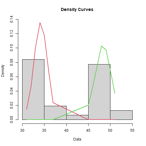
plot(bimodal_fit, density = TRUE, which = 2)
graphics.off()
mtb_add_image("r_bimodal_image.png")
# Now generate tolerance intervals using the parameters found using mixtools
# Set the desired coverage level (e.g., 95%)
coverage_level <- 0.95
alpha <- 1 - coverage_level
# Calculate the tolerance intervals for each component
tolerance_intervals <- lapply(1:2, function(i) {
mu <- bimodal_fit$mu[i]
sigma <- bimodal_fit$sigma[i]
n <- bimodal_fit$lambda[i] # proportion of the component
# Calculate the critical value for the normal distribution
z <- qnorm(1 - alpha / (2 * n))
# Calculate lower and upper bounds of the tolerance interval
lower_bound <- mu - z * sigma
upper_bound <- mu + z * sigma
c(lower_bound, upper_bound)
})
# Show the tolerance intervals
tolerance_intervals_df <- data.frame(
Component = c("First Mode", "Second Mode"),
Lower_Bound = sapply(tolerance_intervals, "[", 1),
Upper_Bound = sapply(tolerance_intervals, "[", 2)
)
myheaders <- c("Component", "Lower Bound", "Upper Bound")
mytitle <- "Tolerance Intervals for Bimodal Distribution"
mtb_add_table(columns = tolerance_intervals_df, headers = myheaders, title = mytitle)
} else {
mtb_add_message("This data is unimodal.")
}
결과
R Script
Modeling a Bimodal Distribution
| Mean | Standard_Deviation | Proportion |
|---|---|---|
| 34.1875 | 1.50909 | 0.516129 |
| 48.3333 | 1.84992 | 0.483871 |
Tolerance Intervals for Bimodal Distribution
| Component | Lower Bound | Upper Bound |
|---|---|---|
| First Mode | 31.6821 | 36.6929 |
| Second Mode | 45.3200 | 51.3467 |