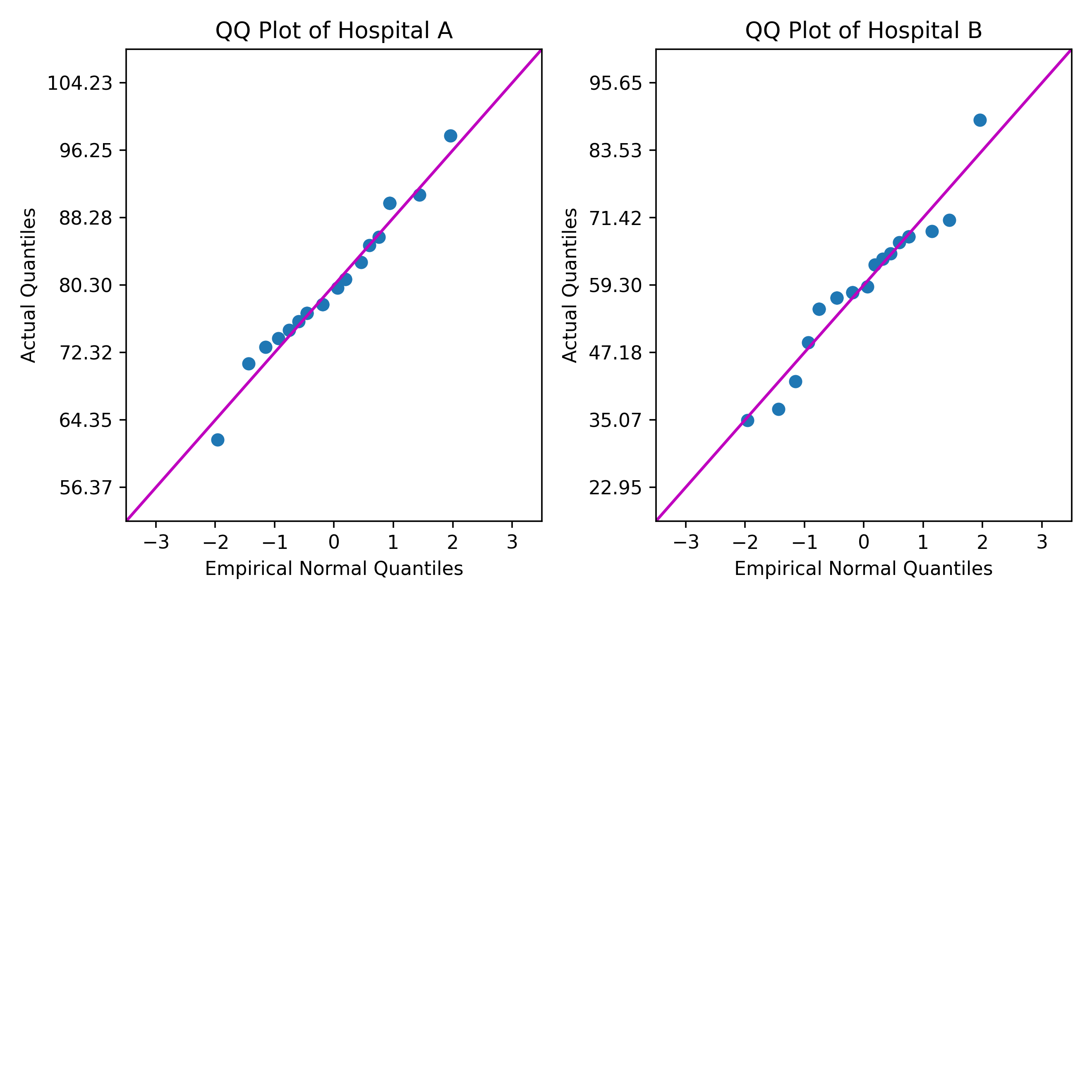
한 의료 컨설턴트는 QQ(quantile-quantile) Plot을 사용하여 두 병원의 환자 만족도 등급의 정규성을 비교하고자 합니다. QQ Plot은 각 환자 만족도 등급 집합이 일반 분포를 얼마나 잘 적합하는지 보여줍니다.
예제 Python 스크립트는 Minitab의 열에서 데이터를 읽습니다. 스크립트는 분위수를 계산하고 각 열에 대한 QQ Plot을 만듭니다. 그런 다음 스크립트가 이 플롯을 Minitab 출력 창으로 보냅니다.
이 가이드에서 참조하는 모든 파일은 .ZIP 파일인 python_guide_files.zip 파일로 제공됩니다.
다음 파일을 사용하여 이 섹션의 단계를 수행합니다.
| 파일 | 설명 |
|---|---|
| qq_plot.py | Minitab 워크시트에서 열을 가져와 각 열에 대한 QQ Plot을 표시하는 Python 스크립트입니다. |
아래 예제의 Python 스크립트에는 다음 Python 모듈이 필요합니다. 괄호 안의 숫자는 스크립트를 실행하는 데 사용한 최신 패키지 버전입니다.
- mtbpy
- Minitab과 Python을 통합하는 Python 모듈입니다. 예제에서는 이 모듈의 함수가 Python 결과를 Minitab으로 보냅니다.
- numpy (1.24.2)
- 과학 및 수치 컴퓨팅을 위한 다양한 응용 프로그램이 있는 Python 모듈입니다.
- matplotlib (3.7.0)
- 그래프 및 그림 생성과 관련된 여러 기능이 있는 Python 모듈입니다.
- 필요한 모듈인 mtbpy 및 numpy를 설치했는지 확인합니다.
- PIP를 통해 필요한 모듈을 설치하려면 운영 체제 터미널(예: Microsoft® Windows Command Prompt 또는 macOS 터미널)에 해당하는 명령을 실행합니다.
pip install mtbpy numpy matplotlib
- PIP를 통해 필요한 모듈을 설치하려면 운영 체제 터미널(예: Microsoft® Windows Command Prompt 또는 macOS 터미널)에 해당하는 명령을 실행합니다.
- Python 스크립트 파일 qq_plot.py를 Minitab 기본 파일 위치에 저장합니다. Minitab이 Python 스크립트 파일을 찾는 위치에 대한 자세한 내용은 Minitab용 Python 파일의 기본 폴더로 이동하십시오.
- 표본 데이터 세트를 엽니다 호텔비교(분할된데이터).MWX.
-
Minitab 명령줄 창에서
PYSC "qq_plot.py" "Hospital A" "Hospital B"을 입력합니다. - 실행을 클릭합니다.
qq_plot.py
"""
Description:
_________________________________________________________________________________
This script will generate a QQ Plot for each column of data passed to PYSC.
If PYSC was not given any columns, the script will look for data in every
column starting with the first column (C1) and ending at the first empty column.
The ranks are calculated using the Modified Kaplan-Meier method,
and duplicate values are given the same rank and quantile, this is also known
as "competition" ranking.
_________________________________________________________________________________
Imports:
_________________________________________________________________________________
numbers - For testing the types of the values in the data columns.
sys - For retrieving any columns passed from Minitab.
statistics - For calculating the inverse CDF of the normal distribution.
numpy - For general calculations and manipulating data.
matplotlib - For creating the plots.
mtbpy - For sending and receiving data with Minitab.
_________________________________________________________________________________
"""
import numbers
import sys
from statistics import NormalDist

import numpy as np
from matplotlib import pyplot as plt
from mtbpy import mtbpy

# sys.argv contains the arguments passed to PYSC, with sys.argv[0] being the name of the Python script file,
# and sys.argv[1:] being the list of columns passed after the name of Python script file,
# sys.argv[1:] has a length of 0 if no columns are passed to the PYSC command.
column_names = sys.argv[1:]

# If column_names is empty, loop over each column, starting at C1, and check if they contain data.
# Stop at the first column that does not contain data, and use the range of columns before that column.
if len(column_names) == 0:
    i = 1
    while mtbpy.mtb_instance().get_column(f"C{i}") is not None:
        column_names.append(f"C{i}")
        i += 1

# If there are no columns to analyze, throw an error stating that columns need to be passed or the data needs to start in C1
if len(column_names) == 0 or mtbpy.mtb_instance().get_column(column_names[0]) is None:
    raise IndexError("Worksheet is empty or column data could not be found!\n\tPass columns to PYSC or move first column to C1.")

# Initialize a list to store data from columns in a list of lists.
columns_data = []
# Loop through each column name.
for column_name in column_names:
    # Use mtbpy to get the data from Minitab for the column as a Python list.
    column_data = mtbpy.mtb_instance().get_column(column_name)
    # If any value in the data is not numeric, throw an error stating that only numeric columns can be used.
    if not all(isinstance(value, numbers.Number) for value in column_data):
        raise ValueError("Data is not numeric!\n\tPass only numeric columns to PYSC or delete non-numeric columns.")
    # Sort the data for calculation of quantiles.
    sorted_column_data = np.sort(column_data)
    # Append the sorted data to our list of column data.
    columns_data.append(sorted_column_data)

# Initialize a figure with:
# Figure Columns = 2 plus the number of data columns modulo 2.
# Figure Rows = Number of data columns floor-divided by the number of figure columns plus 1.
num_plot_cols = 2 + len(columns_data) % 2
num_plot_rows = len(columns_data) // num_plot_cols + 1
fig = plt.figure(figsize=(num_plot_cols * 4, num_plot_rows * 4), tight_layout=True)

# Iterate over the columns and generate a QQ Plot for each column.
for index, column_data in enumerate(columns_data):
    # Create an axis on the figure.
    current_axis = fig.add_subplot(num_plot_rows, num_plot_cols, index + 1)
    # Calculate the quantile of each data point in the column.
    # This uses the Modified Kaplan-Meier ranks, however, the ranks produced by
    # the numpy.searchsorted method begin at "0" and not "1," which would result
    # in negative rank values when using the Modified Kaplan-Meier method.
    # Therefore, the calculation uses rank + 1.0 - 0.5, which simplifies to rank + 0.5.
    column_ranks = np.searchsorted(np.sort(column_data), column_data) + 0.5
    # The quantiles are the ranks divided by the count.
    quantiles = column_ranks / len(column_data)

    # The tick marks on the y-axis and the fit line use the sample mean and sample standard deviation.
    column_mean = np.mean(column_data)
    column_stdev = np.std(column_data)

    # Calculate the empirical quantiles from the normal distribution.
    empirical_quantiles = [NormalDist().inv_cdf(x) for x in quantiles]

    # Create a scatterplot of the sample data versus the empirical quantiles.
    current_axis.scatter(empirical_quantiles, column_data)

    # Create a fit line for a perfect empirical normal distribution, for the scale of this plot, the fit line is 45 degrees.
    current_axis.plot([-3.5, 3.5], [column_mean-3.5*column_stdev, column_mean+3.5*column_stdev], "-m")

    # Set the title for the plot.
    current_axis.set_title(f"QQ Plot of {column_names[index]}")
    # Set the x axis label, bounds, and tick mark positions.
    current_axis.set_xlabel("Empirical Normal Quantiles")
    current_axis.set_xbound(lower=-3.5, upper=3.5)
    current_axis.set_xticks([-3, -2, -1, 0, 1, 2, 3])
    # Set the y axis label, bounds, and tick mark positions.
    current_axis.set_ylabel("Actual Quantiles")
    current_axis.set_ybound(lower=column_mean-3.5*column_stdev,
                            upper=column_mean+3.5*column_stdev)
    current_axis.set_yticks([column_mean-3*column_stdev,
                             column_mean-2*column_stdev,
                             column_mean-1*column_stdev,
                             column_mean,
                             column_mean+1*column_stdev,
                             column_mean+2*column_stdev,
                             column_mean+3*column_stdev])

# Save the combined plots figure as a PNG file.
fig.savefig("qqplot.png", dpi=330)

# Send the figure to Minitab.
mtbpy.mtb_instance().add_image("qqplot.png")
결과
Python Script