エンジン工場の品質エンジニアは、2 つのサプライヤーのピストンのバイモーダル性テストを実行したいと考えています。エンジニアは、各供給業者からの100個のピストンのランダムサンプルの長さを測定します。
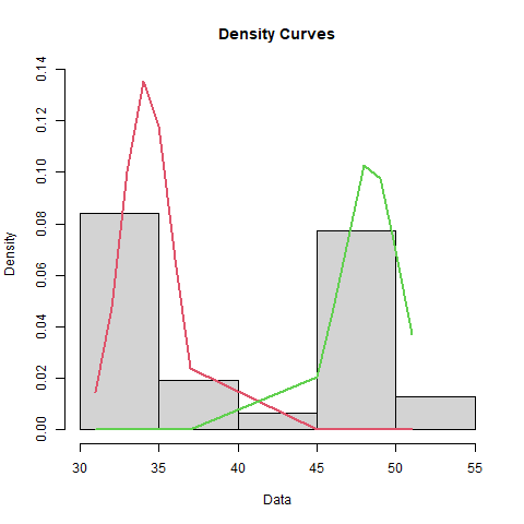
このスクリプトは、R の diptest パッケージを使用して、データがユニモーダルであるかどうかをテストします。検定でユニモーダル データの帰無仮説が棄却された場合、スクリプトはデータが 2 つの正規分布の混合であると仮定します。このスクリプトは、R 用の mixtools パッケージを使用して、2 つの正規分布の記述統計量と密度曲線を表示します。
スクリプト R 例は、統合の次の機能を示しています。
- Minitabワークシートの1つの列を入力として渡します。
- テーブル タイトルを追加します。
- テーブルの列ラベルを追加します。
- テーブルをMinitabの[出力]ペインに送信します。
- グラフを作成し、そのグラフをMinitabの[出力]ペインに送信します。
このセクションの手順を実行するには、次のファイルを使用します。
| ファイル | 説明 |
|---|---|
| bimodal.R | Minitabワークシートから列を取得し、単峰性を検定し、データが単峰性でない場合は2つの正規分布の混合の結果を生成する R スクリプト。 |
このガイドで参照されるすべてのファイルは、次の.ZIPファイルで入手可能です:r_guide_files.zip.
必要条件
-
以下のRスクリプトの例では、以下のRパッケージが必要です:
- mtbr
- MinitabとRを統合するRパッケージ。この例では、このモジュールの関数からR結果がMinitabに送信されます。Minitabの R パッケージのインストール方法については、 手順2を参照してください。 mtbrをインストールします。
- mixtools
- スクリプトが正規分布の混合の出力を作成するために使用する R パッケージ。
- diptest
- データがユニモーダルであるかどうかをテストするためにスクリプトが使用する R パッケージ。
install.packages("mixtools")R パッケージのインストールについては、組織のテクニカル サポート部門にお問い合わせください。Minitabテクニカルサポートは、 R パッケージのインストールをサポートできません。
例を実行する手順
- 次の必要なモジュールがインストールされていることを確認します:mtbr.
- Rスクリプトファイル、bimodal.RをMinitabのデフォルトのファイル位置に保存します。 Minitabが Rスクリプトファイルを探す場所の詳細については、MinitabのRファイルのデフォルトのフォルダを参照してください。
- 工程エネルギーコスト.MWXサンプルデータを開きます。
-
Minitabのコマンドプロンプトペインに、「
RSCR "bimodal.R" "Process 1"」と入力します。 - 実行 を選択します。
bimodal.R
# Load the necessary libraries
#Original code by Valentina Tillman
library(mixtools)
library(mtbr)
library(diptest)

# Retrieve sample data
input_column <- commandArgs(trailingOnly = TRUE)
data <- mtb_get_column(input_column)
dip_test_result <- dip.test(data)

if (dip_test_result$p.value < 0.05) {
  # Fit a bimodal mixture model
  bimodal_fit <- normalmixEM(data, k = 2)

  # Manually extract parameter estimates and format them as a data frame
  bimodal_table <- data.frame(
    Mean = bimodal_fit$mu,
    Standard_Deviation = bimodal_fit$sigma,
    Proportion = bimodal_fit$lambda #tells you what % of the data is clustered around which mean. Also called lambda
  )

  # Define title and headers
  mytitle <- "Modeling a Bimodal Distribution"
  myheaders <- names(bimodal_table)

  # Add the table to the mtbr output
  mtb_add_table(columns = bimodal_table, headers = myheaders, title = mytitle)

  png("r_bimodal_image.png")
  plot(bimodal_fit, density = TRUE, which = 2)
  graphics.off()
  mtb_add_image("r_bimodal_image.png")

  # Now generate tolerance intervals using the parameters found using mixtools
  # Set the desired coverage level (e.g., 95%)
  coverage_level <- 0.95
  alpha <- 1 - coverage_level

  # Calculate the tolerance intervals for each component
  tolerance_intervals <- lapply(1:2, function(i) {
    mu <- bimodal_fit$mu[i]
    sigma <- bimodal_fit$sigma[i]
    n <- bimodal_fit$lambda[i]  # proportion of the component

    # Calculate the critical value for the normal distribution
    z <- qnorm(1 - alpha / (2 * n))

    # Calculate lower and upper bounds of the tolerance interval
    lower_bound <- mu - z * sigma
    upper_bound <- mu + z * sigma

    c(lower_bound, upper_bound)
  })

  # Show the tolerance intervals
  tolerance_intervals_df <- data.frame(
    Component = c("First Mode", "Second Mode"),
    Lower_Bound = sapply(tolerance_intervals, "[", 1),
    Upper_Bound = sapply(tolerance_intervals, "[", 2)
  )

  myheaders <- c("Component", "Lower Bound", "Upper Bound")
  mytitle <- "Tolerance Intervals for Bimodal Distribution"
  mtb_add_table(columns = tolerance_intervals_df, headers = myheaders, title = mytitle)


} else {
  mtb_add_message("This data is unimodal.")
}
結果
R Script
Modeling a Bimodal Distribution
| Mean | Standard_Deviation | Proportion |
|---|---|---|
| 34.1875 | 1.50909 | 0.516129 |
| 48.3333 | 1.84992 | 0.483871 |
Tolerance Intervals for Bimodal Distribution
| Component | Lower Bound | Upper Bound |
|---|---|---|
| First Mode | 31.6821 | 36.6929 |
| Second Mode | 45.3200 | 51.3467 |