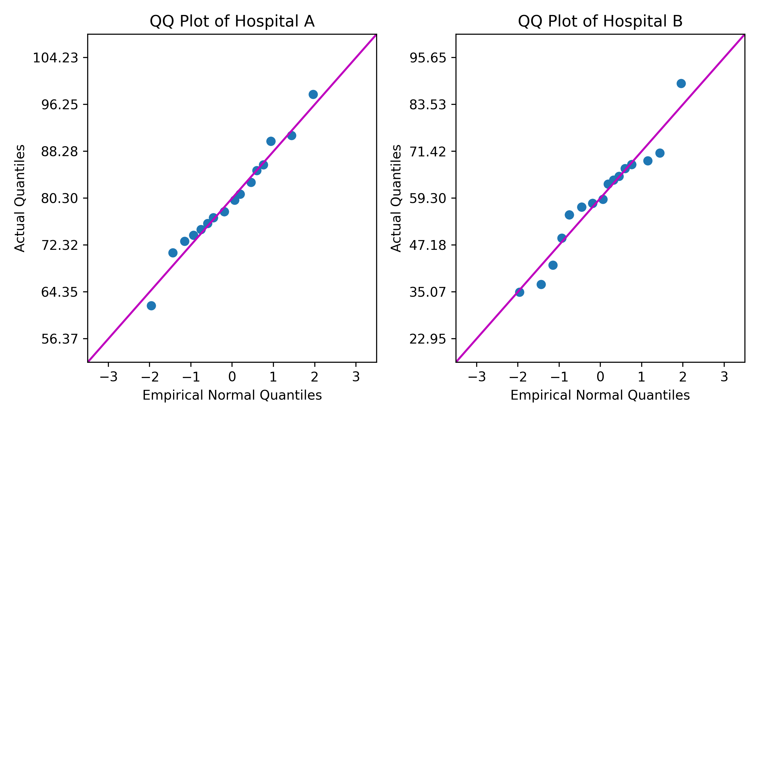
医療コンサルタントは、分位四分位数(QQ)プロットを使用して、2つの病院からの患者満足度評価の正常性を比較したいと考えています。QQプロットは、患者満足度評価の各セットが正規分布にどの程度適合するかを示しています。
この例では、PythonスクリプトがMinitabの列からデータを読み取ります。このスクリプトは、分位数を計算し、各列の QQ プロットを作成します。次に、スクリプトは、Minitab出力ペインにプロットを送信します。
このガイドで参照されるすべてのファイルは、次の.ZIPファイルで入手可能です:python_guide_files.zip.
このセクションの手順を実行するには、次のファイルを使用します。
| ファイル | 説明 |
|---|---|
| qq_plot.py | Minitabワークシートから列を取り出し、各列のQQプロットを表示するPythonスクリプト。 |
次の例のPythonスクリプトには、次のPythonモジュールが必要です。括弧内の数字は、スクリプトの実行に使用した最新のパッケージバージョンです。
- mtbpy
- MinitabとPythonを統合するPythonモジュール。この例では、このモジュールの関数から Python 結果がMinitabに送信されます。
- numpy (1.24.2)
- 科学および数値計算のための様々なアプリケーションを持つPythonモジュール。
- matplotlib (3.7.0)
- グラフのプロットや図の作成に関連するさまざまな関数を持つPythonモジュール。
- 次の必要なモジュールがインストールされていることを確認します:mtbpyおよびnumpy。
- PIPで必要なモジュールをインストールするには、使用するオペレーティングシステムのターミナルに対応するコマンド(Microsoft® Windows Command PromptまたはmacOS Terminalなど)を実行します。
pip install mtbpy numpy matplotlib
- PIPで必要なモジュールをインストールするには、使用するオペレーティングシステムのターミナルに対応するコマンド(Microsoft® Windows Command PromptまたはmacOS Terminalなど)を実行します。
- Pythonスクリプトファイル、qq_plot.pyをMinitabのデフォルトのファイル位置に保存します。 Minitabが Python スクリプトファイルを探す場所の詳細については、MinitabのPythonファイルのデフォルトのフォルダを参照してください。
- ホテル比較非スタック.MWXサンプルデータを開きます。
-
Minitabのコマンドプロンプトペインに、「
PYSC "qq_plot.py" "Hospital A" "Hospital B"」と入力します。 - 実行をクリックします。
qq_plot.py
"""
Description:
_________________________________________________________________________________
This script will generate a QQ Plot for each column of data passed to PYSC.
If PYSC was not given any columns, the script will look for data in every
column starting with the first column (C1) and ending at the first empty column.
The ranks are calculated using the Modified Kaplan-Meier method,
and duplicate values are given the same rank and quantile, this is also known
as "competition" ranking.
_________________________________________________________________________________
Imports:
_________________________________________________________________________________
numbers - For testing the types of the values in the data columns.
sys - For retrieving any columns passed from Minitab.
statistics - For calculating the inverse CDF of the normal distribution.
numpy - For general calculations and manipulating data.
matplotlib - For creating the plots.
mtbpy - For sending and receiving data with Minitab.
_________________________________________________________________________________
"""
import numbers
import sys
from statistics import NormalDist

import numpy as np
from matplotlib import pyplot as plt
from mtbpy import mtbpy

# sys.argv contains the arguments passed to PYSC, with sys.argv[0] being the name of the Python script file,
# and sys.argv[1:] being the list of columns passed after the name of Python script file,
# sys.argv[1:] has a length of 0 if no columns are passed to the PYSC command.
column_names = sys.argv[1:]

# If column_names is empty, loop over each column, starting at C1, and check if they contain data.
# Stop at the first column that does not contain data, and use the range of columns before that column.
if len(column_names) == 0:
    i = 1
    while mtbpy.mtb_instance().get_column(f"C{i}") is not None:
        column_names.append(f"C{i}")
        i += 1

# If there are no columns to analyze, throw an error stating that columns need to be passed or the data needs to start in C1
if len(column_names) == 0 or mtbpy.mtb_instance().get_column(column_names[0]) is None:
    raise IndexError("Worksheet is empty or column data could not be found!\n\tPass columns to PYSC or move first column to C1.")

# Initialize a list to store data from columns in a list of lists.
columns_data = []
# Loop through each column name.
for column_name in column_names:
    # Use mtbpy to get the data from Minitab for the column as a Python list.
    column_data = mtbpy.mtb_instance().get_column(column_name)
    # If any value in the data is not numeric, throw an error stating that only numeric columns can be used.
    if not all(isinstance(value, numbers.Number) for value in column_data):
        raise ValueError("Data is not numeric!\n\tPass only numeric columns to PYSC or delete non-numeric columns.")
    # Sort the data for calculation of quantiles.
    sorted_column_data = np.sort(column_data)
    # Append the sorted data to our list of column data.
    columns_data.append(sorted_column_data)

# Initialize a figure with:
# Figure Columns = 2 plus the number of data columns modulo 2.
# Figure Rows = Number of data columns floor-divided by the number of figure columns plus 1.
num_plot_cols = 2 + len(columns_data) % 2
num_plot_rows = len(columns_data) // num_plot_cols + 1
fig = plt.figure(figsize=(num_plot_cols * 4, num_plot_rows * 4), tight_layout=True)

# Iterate over the columns and generate a QQ Plot for each column.
for index, column_data in enumerate(columns_data):
    # Create an axis on the figure.
    current_axis = fig.add_subplot(num_plot_rows, num_plot_cols, index + 1)
    # Calculate the quantile of each data point in the column.
    # This uses the Modified Kaplan-Meier ranks, however, the ranks produced by
    # the numpy.searchsorted method begin at "0" and not "1," which would result
    # in negative rank values when using the Modified Kaplan-Meier method.
    # Therefore, the calculation uses rank + 1.0 - 0.5, which simplifies to rank + 0.5.
    column_ranks = np.searchsorted(np.sort(column_data), column_data) + 0.5
    # The quantiles are the ranks divided by the count.
    quantiles = column_ranks / len(column_data)

    # The tick marks on the y-axis and the fit line use the sample mean and sample standard deviation.
    column_mean = np.mean(column_data)
    column_stdev = np.std(column_data)

    # Calculate the empirical quantiles from the normal distribution.
    empirical_quantiles = [NormalDist().inv_cdf(x) for x in quantiles]

    # Create a scatterplot of the sample data versus the empirical quantiles.
    current_axis.scatter(empirical_quantiles, column_data)

    # Create a fit line for a perfect empirical normal distribution, for the scale of this plot, the fit line is 45 degrees.
    current_axis.plot([-3.5, 3.5], [column_mean-3.5*column_stdev, column_mean+3.5*column_stdev], "-m")

    # Set the title for the plot.
    current_axis.set_title(f"QQ Plot of {column_names[index]}")
    # Set the x axis label, bounds, and tick mark positions.
    current_axis.set_xlabel("Empirical Normal Quantiles")
    current_axis.set_xbound(lower=-3.5, upper=3.5)
    current_axis.set_xticks([-3, -2, -1, 0, 1, 2, 3])
    # Set the y axis label, bounds, and tick mark positions.
    current_axis.set_ylabel("Actual Quantiles")
    current_axis.set_ybound(lower=column_mean-3.5*column_stdev,
                            upper=column_mean+3.5*column_stdev)
    current_axis.set_yticks([column_mean-3*column_stdev,
                             column_mean-2*column_stdev,
                             column_mean-1*column_stdev,
                             column_mean,
                             column_mean+1*column_stdev,
                             column_mean+2*column_stdev,
                             column_mean+3*column_stdev])

# Save the combined plots figure as a PNG file.
fig.savefig("qqplot.png", dpi=330)

# Send the figure to Minitab.
mtbpy.mtb_instance().add_image("qqplot.png")
結果
Python Script