In This Topic
Effect
An effect describes the size and direction of the relationship between a term and the response variable. Minitab calculates effects for factors and interactions among factors.
Interpretation
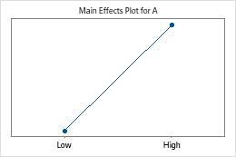
The effect for a factor represents the predicted change in the mean response when the factor changes from the low level to the high level. Effects are twice the value of the coded coefficients. The sign of the effect indicates the direction of the relationship between the term and the response.
With more factors in an interaction, you have more difficulty interpreting the effect. For factors and interactions among factors, the size of the effect is usually a good way to assess the practical significance of the effect that a term has on the response variable.
The size of the effect does not indicate whether a term is statistically significant because the calculations for significance also consider the variation in the response data. To determine statistical significance, examine the p-value for the term.
Ratio effect
Ratio effects can provide a measure of the practical significance of a factor's effect. The ratio effect indicates the proportional increase or decrease in the standard deviation of the response when the factor is changed from the low to high level. The closer the ratio effect is to one, the smaller the effect of the factor.
The ratio effect estimates the ratio of the standard deviation of responses at the high level of the factor to the standard deviation of responses at the low level of the factor. The ratio effect is easily calculated by exponentiating the effect of a factor.
Interpretation
- For material, the ratio effect is 0.3830. This means that when the insulation uses formula 2 the standard deviation is 38% of the value when the insulation is formula 1. Because the material by injection pressure interaction is significant, the main effect for material cannot be interpreted without considering the interaction effect.
- For the material by injection pressure interaction, the ratio effect is 0.3709.
To predict the result of changing material from formula 1 to formula 2 while keeping injection pressure the same, multiply or divide the ratio effect for material by the ratio effect for the interaction. If injection pressure is at its low level, then divide the ratio effect for material by the ratio effect for the interaction to get 0.3830/0.3709 = 1.0326, is a small increase in the standard deviation of about 3%. If injection pressure is at the high level, multiply the two ratio effects to get 0.3830 * 0.3709 = 0.1421, a reduction in the standard deviation of over 85% (1 – 0.1421 = 0.8579).
When both factors are set at their low levels (or at their high levels) then the interaction term is at its high level (−1 * −1 = 1; 1 * 1 = 1). Remember, −1 is the low level and 1 is the high level. When one factor is set at the high level and the other set at the low level, then the interaction term is at the low level (−1 * 1 = −1). Changing material from low to high while keeping injection pressure low changes the interaction term from high to low. The two ratios work in opposite directions, and you divide them to determine the effect. If injection pressure is high, then changing material from low to high also changes the interaction term from low to high. The ratios work in the same direction, and you multiply them to determine the effect.
Coded Coefficients for Ln(Std)
| Term | Effect | Ratio Effect | Coef | SE Coef | T-Value | P-Value | VIF |
|---|---|---|---|---|---|---|---|
| Constant | 0.3424 | 0.0481 | 7.12 | 0.001 | |||
| Material | -0.9598 | 0.3830 | -0.4799 | 0.0481 | -9.99 | 0.000 | 1.00 |
| InjPress | -0.1845 | 0.8315 | -0.0922 | 0.0481 | -1.92 | 0.113 | 1.00 |
| InjTemp | 0.0555 | 1.0571 | 0.0278 | 0.0481 | 0.58 | 0.589 | 1.00 |
| CoolTemp | -0.1259 | 0.8817 | -0.0629 | 0.0481 | -1.31 | 0.247 | 1.00 |
| Material*InjPress | -0.9918 | 0.3709 | -0.4959 | 0.0481 | -10.32 | 0.000 | 1.00 |
| Material*InjTemp | 0.1875 | 1.2062 | 0.0937 | 0.0481 | 1.95 | 0.109 | 1.00 |
| Material*CoolTemp | 0.0056 | 1.0056 | 0.0028 | 0.0481 | 0.06 | 0.956 | 1.00 |
| InjPress*InjTemp | -0.0792 | 0.9239 | -0.0396 | 0.0481 | -0.82 | 0.448 | 1.00 |
| InjPress*CoolTemp | -0.0900 | 0.9139 | -0.0450 | 0.0481 | -0.94 | 0.392 | 1.00 |
| InjTemp*CoolTemp | 0.0066 | 1.0066 | 0.0033 | 0.0481 | 0.07 | 0.948 | 1.00 |
Coef
The coefficient describes the size and direction of the relationship between a term in the model and the response variable. To minimize multicollinearity among the terms, the coefficients are all in coded units.
Interpretation
The coefficient for a term represents the change in the mean response associated with an increase of one coded unit in that term, while the other terms are held constant. The sign of the coefficient indicates the direction of the relationship between the term and the response.
The size of the coefficient is half the size of the effect. The effect represents the change in the predicted mean response when a factor changes from its low level to its high level.
The size of the effect is usually a good way to assess the practical significance of the effect that a term has on the response variable. The size of the effect does not indicate whether a term is statistically significant because the calculations for significance also consider the variation in the response data. To determine statistical significance, examine the p-value for the term.
- Covariates
- The coefficient for a covariate is in the same units as the covariate. The coefficient represents the change in the predicted mean of the response for a one unit increase in the covariate. If the coefficient is negative, as the covariate increases, the predicted mean of the response decreases. If the coefficient is positive, as the covariate increases, the predicted mean of the response increases. Because covariates are not coded and are not usually orthogonal to the factors, the presence of covariates usually increases VIF values. For more information, go to the section on VIF.
- Blocks
- Blocks are categorical variables with a (−1, 0, +1) coding scheme. Each coefficient represents the difference between the mean of the response for the block and the overall mean of the response.
- CenterPt
- Center points are a categorical variable with a (0, 1) coding scheme. The reference level is when the categorical variable equals 1, which is for data at the factorial points of the design. The categorical variable is 0 at the center points of the design. Usually, you use the p-value to determine the value of further data collection to estimate quadratic effects of the factors. Usually, you do not interpret the coefficient of the CenterPt term because the term represents as many aliased quadratic effects as factors in the design.
SE Coef
The standard error of the coefficient estimates the variability between coefficient estimates that you would obtain if you took samples from the same population again and again. The calculation assumes that the experimental design and the coefficients to estimate would remain the same if you sampled again and again.
Interpretation
Use the standard error of the coefficient to measure the precision of the estimate of the coefficient. The smaller the standard error, the more precise the estimate. Dividing the coefficient by its standard error calculates a t-value. If the p-value associated with this t-statistic is less than your significance level, you conclude that the coefficient is statistically significant.
T-value
The t-value measures the ratio between the coefficient and its standard error.
Interpretation
Minitab uses the t-value to calculate the p-value, which you use to test whether the coefficient is significantly different from 0.
You can use the t-value to determine whether to reject the null hypothesis. However, the p-value is used more often because the threshold for the rejection of the null hypothesis does not depend on the degrees of freedom. For more information on using the t-value, go to Using the t-value to determine whether to reject the null hypothesis.
Confidence Interval for coefficient (95% CI)
These confidence intervals (CI) are ranges of values that are likely to contain the true value of the coefficient for each term in the model.
Because samples are random, two samples from a population are unlikely to yield identical confidence intervals. However, if you take many random samples, a certain percentage of the resulting confidence intervals contain the unknown population parameter. The percentage of these confidence intervals that contain the parameter is the confidence level of the interval.
- Point estimate
- This single value estimates a population parameter by using your sample data. The confidence interval is centered around the point estimate.
- Margin of error
- The margin of error defines the width of the confidence interval and is determined by the observed variability in the sample, the sample size, and the confidence level. To calculate the upper limit of the confidence interval, the margin of error is added to the point estimate. To calculate the lower limit of the confidence interval, the margin of error is subtracted from the point estimate.
Interpretation
Use the confidence interval to assess the estimate of the population coefficient for each term in the model.
For example, with a 95% confidence level, you can be 95% confident that the confidence interval contains the value of the coefficient for the population. The confidence interval helps you assess the practical significance of your results. Use your specialized knowledge to determine whether the confidence interval includes values that have practical significance for your situation. If the interval is too wide to be useful, consider increasing your sample size.
Z-Value
The Z-value is a test statistic that measures the ratio between the coefficient and its standard error. The Z-value is display when you use the maximum likelihood method of estimation.
Interpretation
Minitab uses the Z-value to calculate the p-value, which you use to make a decision about the statistical significance of the terms and the model.
A Z-value that is sufficiently far from 0 indicates that the coefficient estimate is both large and precise enough to be statistically different from 0. Conversely, a Z-value that is close to 0 indicates that the coefficient estimate is too small or too imprecise to be certain that the term has an effect on the response.
P-Value – Coefficient
The p-value is a probability that measures the evidence against the null hypothesis. Lower probabilities provide stronger evidence against the null hypothesis.
Interpretation
To determine whether a coefficient is statistically different from 0, compare the p-value for the term to your significance level to assess the null hypothesis. The null hypothesis is that the coefficient equals 0, which implies that there is no association between the term and the response.
Usually, a significance level (denoted as α or alpha) of 0.05 works well. A significance level of 0.05 indicates a 5% risk of concluding that the coefficient is not 0 when it is.
- P-value ≤ α: The association is statistically significant
- If the p-value is less than or equal to the significance level, you can conclude that there is a statistically significant association between the response variable and the term.
- P-value > α: The association is not statistically significant
- If the p-value is greater than the significance level, you cannot conclude that there is a statistically significant association between the response variable and the term. You may want to refit the model without the term.
- Factors
- If the coefficient for a factor is statistically significant, you can conclude that the coefficient for the factor does not equal 0.
- Interactions among factors
- If the coefficient for an interaction is statistically significant, you can conclude that the relationship between a factor and the response depends on the other factors in the term.
- Covariates
- If the coefficient for a covariate is statistically significant, you can conclude that the association between the response and the covariate is statistically significant.
- Blocks
- If the coefficient for a block is statistically significant, you can conclude that the mean of the response values in that block is different from the overall mean of the response.
- CenterPt
- If the coefficient for a center point is statistically significant, you can conclude that at least one of the factors has a curved relationship with the response. You may want to add axial points to the design so that you can model the curvature.
VIF
The variance inflation factor (VIF) indicates how much the variance of a coefficient is inflated due to correlations among the predictors in the model.
Interpretation
Use the VIF to describe how much multicollinearity (which is correlation between predictors) exists in a model. All the VIF values are 1 in most factorial designs, which indicates the predictors have no multicollinearity. The absence of multicollinearity simplifies the determination of statistical significance. The inclusion of covariates in the model and the occurrence of botched runs during data collection are two common ways that VIF values increase, which complicates the interpretation of statistical significance. Also for binary responses, the VIF values are often greater than 1.
| VIF | Status of predictor |
|---|---|
| VIF = 1 | Not correlated |
| 1 < VIF < 5 | Moderately correlated |
| VIF > 5 | Highly correlated |
- Coefficients can seem to be not statistically significant even when an important relationship exists between the predictor and the response.
- Coefficients for highly correlated predictors will vary widely from sample to sample.
- Removing any highly correlated terms from the model will greatly affect the estimated coefficients of the other highly correlated terms. Coefficients of the highly correlated terms can even change direction of the effect.
Be cautious when you use statistical significance to choose terms to remove from a model in the presence of multicollinearity. Add and remove only one term at a time from the model. Monitor changes in the model summary statistics, as well as the tests of statistical significance, as you change the model.