In This Topic
Null hypothesis and alternative hypothesis
- Null hypothesis
- The null hypothesis states that a population parameter (such as the mean, the standard deviation, and so on) is equal to a hypothesized value. The null hypothesis is often an initial claim that is based on previous analyses or specialized knowledge.
- Alternative hypothesis
- The alternative hypothesis states that a population parameter is smaller, larger, or different from the hypothesized value in the null hypothesis. The alternative hypothesis is what you might believe to be true or hope to prove true.
In the output, the null and alternative hypotheses help you to verify that you entered the correct value for the hypothesized mean.
N
The sample size (N) is the total number of observations in the sample.
Interpretation
The sample size affects the confidence interval and the power of the test.
Usually, a larger sample size results in a narrower confidence interval. A larger sample size also gives the test more power to detect a difference. For more information, go to What is power?.
Mean
The mean summarizes the sample values with a single value that represents the center of the data. The mean is the average of the data, which is the sum of all the observations divided by the number of observations.
Interpretation
The mean of the sample data is an estimate of the population mean.
Because the mean is based on sample data and not on the entire population, it is unlikely that the sample mean equals the population mean. To better estimate the population mean, use the confidence interval.
StDev
The standard deviation is the most common measure of dispersion, or how spread out the data are about the mean. The symbol σ (sigma) is often used to represent the standard deviation of a population, while s is used to represent the standard deviation of a sample. Variation that is random or natural to a process is often referred to as noise.
The standard deviation uses the same units as the data.
Interpretation
Use the standard deviation to determine how spread out the data are from the mean. A higher standard deviation value indicates greater spread in the data. A good rule of thumb for a normal distribution is that approximately 68% of the values fall within one standard deviation of the mean, 95% of the values fall within two standard deviations, and 99.7% of the values fall within three standard deviations.
The standard deviation of the sample data is an estimate of the population standard deviation. The standard deviation is used to calculate the confidence interval and the p-value. A higher value produces less precise (wider) confidence intervals and less powerful tests.
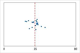
Hospital 1
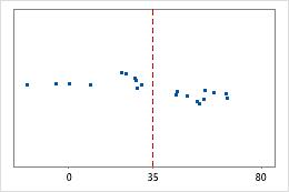
Hospital 2
Hospital discharge times
Administrators track the discharge time for patients who are treated in the emergency departments of two hospitals. Although the average discharge times are about the same (35 minutes), the standard deviations are significantly different. The standard deviation for hospital 1 is about 6. On average, a patient's discharge time deviates from the mean (dashed line) by about 6 minutes. The standard deviation for hospital 2 is about 20. On average, a patient's discharge time deviates from the mean (dashed line) by about 20 minutes.
SE mean
The standard error of the mean (SE Mean) estimates the variability between sample means that you would obtain if you took repeated samples from the same population. Whereas the standard error of the mean estimates the variability between samples, the standard deviation measures the variability within a single sample.
For example, you have a mean delivery time of 3.80 days, with a standard deviation of 1.43 days, from a random sample of 312 delivery times. These numbers yield a standard error of the mean of 0.08 days (1.43 divided by the square root of 312). If you took multiple random samples of the same size, from the same population, the standard deviation of those different sample means would be around 0.08 days.
Interpretation
Use the standard error of the mean to determine how precisely the sample mean estimates the population mean.
A smaller value of the standard error of the mean indicates a more precise estimate of the population mean. Usually, a larger standard deviation results in a larger standard error of the mean and a less precise estimate of the population mean. A larger sample size results in a smaller standard error of the mean and a more precise estimate of the population mean.
Minitab uses the standard error of the mean to calculate the confidence interval.
Confidence interval (CI) and bounds
The confidence interval provides a range of likely values for the population mean. Because samples are random, two samples from a population are unlikely to yield identical confidence intervals. But, if you repeated your sample many times, a certain percentage of the resulting confidence intervals or bounds would contain the unknown population mean. The percentage of these confidence intervals or bounds that contain the mean is the confidence level of the interval. For example, a 95% confidence level indicates that if you take 100 random samples from the population, you could expect approximately 95 of the samples to produce intervals that contain the population mean.
An upper bound defines a value that the population mean is likely to be less than. A lower bound defines a value that the population mean is likely to be greater than.
The confidence interval helps you assess the practical significance of your results. Use your specialized knowledge to determine whether the confidence interval includes values that have practical significance for your situation. If the interval is too wide to be useful, consider increasing your sample size. For more information, go to Ways to get a more precise confidence interval.
Descriptive Statistics
| N | Mean | StDev | SE Mean | 95% CI for μ |
|---|---|---|---|---|
| 25 | 330.6 | 154.2 | 30.8 | (266.9, 394.2) |
In these results, the estimate of the population mean for energy cost is 330.6. You can be 95% confident that the population mean is between 266.9 and 394.2.
T-Value
The t-value is the observed value of the t-test statistic that measures the difference between an observed sample statistic and its hypothesized population parameter, in units of standard error.
Interpretation
You can compare the t-value to critical values of the t-distribution to determine whether to reject the null hypothesis. However, using the p-value of the test to make the same determination is usually more practical and convenient.
To determine whether to reject the null hypothesis, compare the t-value to the critical value. The critical value is tα/2, n–1 for a two-sided test and tα, n–1 for a one-sided test. For a two-sided test, if the absolute value of the t-value is greater than the critical value, you reject the null hypothesis. If it is not, you fail to reject the null hypothesis. You can calculate the critical value in Minitab or find the critical value from a t-distribution table in most statistics books. For more information, go to Using the inverse cumulative distribution function (ICDF) and click "Use the ICDF to calculate critical values".
P-Value
The p-value is a probability that measures the evidence against the null hypothesis. A smaller p-value provides stronger evidence against the null hypothesis.
Interpretation
Use the p-value to determine whether the population mean is statistically different from the hypothesized mean.
- P-value ≤ α: The difference between the means is statistically significant (Reject H0)
- If the p-value is less than or equal to the significance level, the decision is to reject the null hypothesis. You can conclude that the difference between the population mean and the hypothesized mean is statistically significant. Use your specialized knowledge to determine whether the difference is practically significant. For more information, go to Statistical and practical significance.
- P-value > α: The difference between the means is not statistically significant (Fail to reject H0)
- If the p-value is greater than the significance level, the decision is to fail to reject the null hypothesis. You do not have enough evidence to conclude that the difference between the population mean and the hypothesized mean is statistically significant. You should make sure that your test has enough power to detect a difference that is practically significant. For more information, go to Power and Sample Size for 1-Sample t.
Histogram
A histogram divides sample values into many intervals and represents the frequency of data values in each interval with a bar.
Interpretation
Use a histogram to assess the shape and spread of the data. Histograms are best when the sample size is greater than 20.
- Skewed data
-
Examine the spread of your data to determine whether your data appear to be skewed. When data are skewed, the majority of the data are located on the high or low side of the graph. Often, skewness is easiest to detect with a histogram or boxplot.
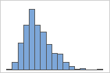
Right-skewed
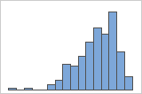
Left-skewed
The histogram with right-skewed data shows wait times. Most of the wait times are relatively short, and only a few wait times are long. The histogram with left-skewed data shows failure time data. A few items fail immediately, and many more items fail later.
Data that are severely skewed can affect the validity of the p-value if your sample is small (less than 20 values). If your data are severely skewed and you have a small sample, consider increasing your sample size.
- Outliers
-
Outliers, which are data values that are far away from other data values, can strongly affect the results of your analysis. Often, outliers are easiest to identify on a boxplot.
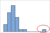
On a histogram, isolated bars at either ends of the graph identify possible outliers.
Try to identify the cause of any outliers. Correct any data–entry errors or measurement errors. Consider removing data values for abnormal, one-time events (also called special causes). Then, repeat the analysis. For more information, go to Identifying outliers.
Individual value plot
An individual value plot displays the individual values in the sample. Each circle represents one observation. An individual value plot is especially useful when you have relatively few observations and when you also need to assess the effect of each observation.
Interpretation
Use an individual value plot to examine the spread of the data and to identify any potential outliers. Individual value plots are best when the sample size is less than 50.
- Skewed data
-
Examine the spread of your data to determine whether your data appear to be skewed. When data are skewed, the majority of the data are located on the high or low side of the graph. Often, skewness is easiest to detect with a histogram or boxplot.
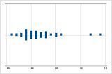
Right-skewed
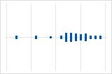
Left-skewed
The individual value plot with right-skewed data shows wait times. Most of the wait times are relatively short, and only a few wait times are long. The individual value plot with left-skewed data shows failure time data. A few items fail immediately, and many more items fail later.
Data that are severely skewed can affect the validity of the p-value if your sample is small (less than 20 values). If your data are severely skewed and you have a small sample, consider increasing your sample size.
- Outliers
-
Outliers, which are data values that are far away from other data values, can strongly affect the results of your analysis. Often, outliers are easiest to identify on a boxplot.
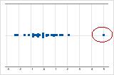
On an individual value plot, unusually low or high data values indicate possible outliers.
Try to identify the cause of any outliers. Correct any data–entry errors or measurement errors. Consider removing data values for abnormal, one-time events (also called special causes). Then, repeat the analysis. For more information, go to Identifying outliers.
Boxplot
A boxplot provides a graphical summary of the distribution of a sample. The boxplot shows the shape, central tendency, and variability of the data.
Interpretation
Use a boxplot to examine the spread of the data and to identify any potential outliers. Boxplots are best when the sample size is greater than 20.
- Skewed data
-
Examine the spread of your data to determine whether your data appear to be skewed. When data are skewed, the majority of the data are located on the high or low side of the graph. Often, skewness is easiest to detect with a histogram or boxplot.
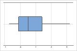
Right-skewed
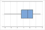
Left-skewed
The boxplot with right-skewed data shows wait times. Most of the wait times are relatively short, and only a few wait times are long. The boxplot with left-skewed data shows failure time data. A few items fail immediately, and many more items fail later.
Data that are severely skewed can affect the validity of the p-value if your sample is small (less than 20 values). If your data are severely skewed and you have a small sample, consider increasing your sample size.
- Outliers
-
Outliers, which are data values that are far away from other data values, can strongly affect the results of your analysis. Often, outliers are easiest to identify on a boxplot.
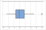
On a boxplot, asterisks (*) denote outliers.
Try to identify the cause of any outliers. Correct any data–entry errors or measurement errors. Consider removing data values for abnormal, one-time events (also called special causes). Then, repeat the analysis. For more information, go to Identifying outliers.