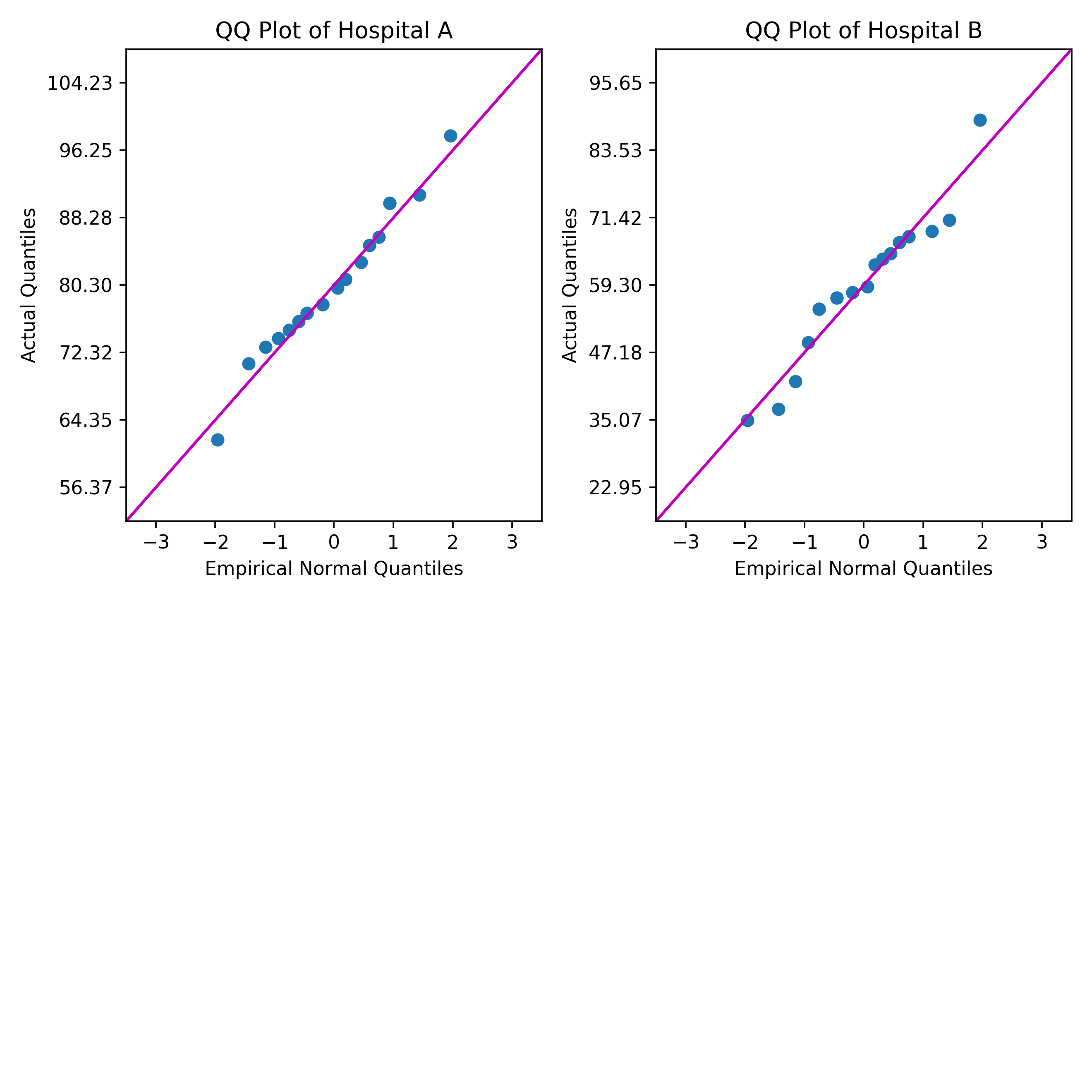
Un consultant dans le domaine de la santé souhaite comparer le niveau de satisfaction des patients de deux hôpitaux à l'aide d'un diagramme quantile-quantile (QQ). Les diagrammes QQ montrent dans quelle mesure chaque ensemble de niveau de satisfaction des patients s'ajuste à une loi normale.
L'exemple de script Python lit les données des colonnes de Minitab. Le script calcule les quantiles et crée un diagramme QQ pour chaque colonne. Il envoie ensuite les diagrammes vers le panneau des résultats de Minitab.
Tous les fichiers référencés dans ce guide sont disponibles dans ce fichier .ZIP : python_guide_files.zip.
Utilisez les fichiers suivants pour effectuer les étapes de cette section :
| Fichier | Description |
|---|---|
| qq_plot.py | Script Python qui utilise des colonnes d'une feuille de travail Minitab pour afficher le diagramme QQ pour chaque colonne. |
Le script Python dans l'exemple ci-dessous exige les modules Python suivants. Le nombre entre parenthèses est la version de package la plus récente que nous avons utilisée pour exécuter le script.
- mtbpy
- Module Python qui intègre Minitab et Python. Dans l'exemple, les fonctions de ce module envoient les résultats Python à Minitab.
- numpy (1.24.2)
- Module Python qui présente diverses applications pour les calculs scientifiques et numériques.
- matplotlib (3.7.0)
- Module Python qui présente diverses fonctions liées à la création de graphiques et de figures.
- Vérifiez que vous avez installé les modules exigés : mtbpy et numpy.
- Pour installer les modules requis via PIP, exécutez la commande correspondante pour le terminal de votre système d'exploitation (par exemple, Microsoft® Windows Command Prompt ou le terminal macOS) :
pip install mtbpy numpy matplotlib
- Pour installer les modules requis via PIP, exécutez la commande correspondante pour le terminal de votre système d'exploitation (par exemple, Microsoft® Windows Command Prompt ou le terminal macOS) :
- Enregistrez le fichier de script Python, qq_plot.py, à votre emplacement de fichier par défaut Minitab. Pour plus d’informations sur l'emplacement où Minitab Python recherche des fichiers de script, allez dans Dossiers par défaut pour les fichiers Python pour Minitab.
- Ouvrez l'ensemble de données échantillons DonnéesDésempiléesSurLaComparaisonD'hôpitaux.MWX.
-
Dans le panneau Minitab Ligne de
commande, saisissez
PYSC "qq_plot.py" "Hospital A" "Hospital B". - Cliquez sur Essai.
qq_plot.py
"""
Description:
_________________________________________________________________________________
This script will generate a QQ Plot for each column of data passed to PYSC.
If PYSC was not given any columns, the script will look for data in every
column starting with the first column (C1) and ending at the first empty column.
The ranks are calculated using the Modified Kaplan-Meier method,
and duplicate values are given the same rank and quantile, this is also known
as "competition" ranking.
_________________________________________________________________________________
Imports:
_________________________________________________________________________________
numbers - For testing the types of the values in the data columns.
sys - For retrieving any columns passed from Minitab.
statistics - For calculating the inverse CDF of the normal distribution.
numpy - For general calculations and manipulating data.
matplotlib - For creating the plots.
mtbpy - For sending and receiving data with Minitab.
_________________________________________________________________________________
"""
import numbers
import sys
from statistics import NormalDist

import numpy as np
from matplotlib import pyplot as plt
from mtbpy import mtbpy

# sys.argv contains the arguments passed to PYSC, with sys.argv[0] being the name of the Python script file,
# and sys.argv[1:] being the list of columns passed after the name of Python script file,
# sys.argv[1:] has a length of 0 if no columns are passed to the PYSC command.
column_names = sys.argv[1:]

# If column_names is empty, loop over each column, starting at C1, and check if they contain data.
# Stop at the first column that does not contain data, and use the range of columns before that column.
if len(column_names) == 0:
    i = 1
    while mtbpy.mtb_instance().get_column(f"C{i}") is not None:
        column_names.append(f"C{i}")
        i += 1

# If there are no columns to analyze, throw an error stating that columns need to be passed or the data needs to start in C1
if len(column_names) == 0 or mtbpy.mtb_instance().get_column(column_names[0]) is None:
    raise IndexError("Worksheet is empty or column data could not be found!\n\tPass columns to PYSC or move first column to C1.")

# Initialize a list to store data from columns in a list of lists.
columns_data = []
# Loop through each column name.
for column_name in column_names:
    # Use mtbpy to get the data from Minitab for the column as a Python list.
    column_data = mtbpy.mtb_instance().get_column(column_name)
    # If any value in the data is not numeric, throw an error stating that only numeric columns can be used.
    if not all(isinstance(value, numbers.Number) for value in column_data):
        raise ValueError("Data is not numeric!\n\tPass only numeric columns to PYSC or delete non-numeric columns.")
    # Sort the data for calculation of quantiles.
    sorted_column_data = np.sort(column_data)
    # Append the sorted data to our list of column data.
    columns_data.append(sorted_column_data)

# Initialize a figure with:
# Figure Columns = 2 plus the number of data columns modulo 2.
# Figure Rows = Number of data columns floor-divided by the number of figure columns plus 1.
num_plot_cols = 2 + len(columns_data) % 2
num_plot_rows = len(columns_data) // num_plot_cols + 1
fig = plt.figure(figsize=(num_plot_cols * 4, num_plot_rows * 4), tight_layout=True)

# Iterate over the columns and generate a QQ Plot for each column.
for index, column_data in enumerate(columns_data):
    # Create an axis on the figure.
    current_axis = fig.add_subplot(num_plot_rows, num_plot_cols, index + 1)
    # Calculate the quantile of each data point in the column.
    # This uses the Modified Kaplan-Meier ranks, however, the ranks produced by
    # the numpy.searchsorted method begin at "0" and not "1," which would result
    # in negative rank values when using the Modified Kaplan-Meier method.
    # Therefore, the calculation uses rank + 1.0 - 0.5, which simplifies to rank + 0.5.
    column_ranks = np.searchsorted(np.sort(column_data), column_data) + 0.5
    # The quantiles are the ranks divided by the count.
    quantiles = column_ranks / len(column_data)

    # The tick marks on the y-axis and the fit line use the sample mean and sample standard deviation.
    column_mean = np.mean(column_data)
    column_stdev = np.std(column_data)

    # Calculate the empirical quantiles from the normal distribution.
    empirical_quantiles = [NormalDist().inv_cdf(x) for x in quantiles]

    # Create a scatterplot of the sample data versus the empirical quantiles.
    current_axis.scatter(empirical_quantiles, column_data)

    # Create a fit line for a perfect empirical normal distribution, for the scale of this plot, the fit line is 45 degrees.
    current_axis.plot([-3.5, 3.5], [column_mean-3.5*column_stdev, column_mean+3.5*column_stdev], "-m")

    # Set the title for the plot.
    current_axis.set_title(f"QQ Plot of {column_names[index]}")
    # Set the x axis label, bounds, and tick mark positions.
    current_axis.set_xlabel("Empirical Normal Quantiles")
    current_axis.set_xbound(lower=-3.5, upper=3.5)
    current_axis.set_xticks([-3, -2, -1, 0, 1, 2, 3])
    # Set the y axis label, bounds, and tick mark positions.
    current_axis.set_ylabel("Actual Quantiles")
    current_axis.set_ybound(lower=column_mean-3.5*column_stdev,
                            upper=column_mean+3.5*column_stdev)
    current_axis.set_yticks([column_mean-3*column_stdev,
                             column_mean-2*column_stdev,
                             column_mean-1*column_stdev,
                             column_mean,
                             column_mean+1*column_stdev,
                             column_mean+2*column_stdev,
                             column_mean+3*column_stdev])

# Save the combined plots figure as a PNG file.
fig.savefig("qqplot.png", dpi=330)

# Send the figure to Minitab.
mtbpy.mtb_instance().add_image("qqplot.png")
Résultats
Python Script