In This Topic
- Lot quality
- Lower specification limit (LSL) and upper specification limit (USL)
- Historical standard deviation
- Lot size
- Acceptable quality level (AQL) and Rejectable quality level (RQL or LTPD)
- Producer's Risk (Alpha) and Consumer's Risk (Beta)
- Sample size
- Critical distance (k value)
- Maximum standard deviation (MSD)
Lot quality
- Percent defective
- Represents the percentage defective as a value between 0 and 100. For example, if 10 units are defective out of a sample size of 500, the percent defective is 2.
- Proportion defective
- Represents the proportion defective as a value between 0 and 1. For example, if 10 units are defective out of a sample size of 500, the proportion defective is 0.02.
- Defectives per million
- Represents the level of defectives as a value out of a million units. For example, 10 defectives per million (DPM) means that you have 10 defective units for every million units.
Lower specification limit (LSL) and upper specification limit (USL)
The lower specification limit (LSL) is the minimum allowed value for the product or service. This limit does not indicate how the process is performing but how you want it to perform.
The upper specification limit (USL) is the maximum allowed value for the product or service. This limit does not indicate how the process is performing but how you want it to perform.
You must specify at least one specification limit for a variables acceptance sampling plan.
Interpretation
Use the LSL and USL to define customer requirements and to evaluate whether your process produces items that meet the requirements.
Minitab compares your process data to the specification limits to determine whether to accept or reject an entire lot of product.
Historical standard deviation
The historical standard deviation is the known standard deviation of your process. Use a historical standard deviation when you have collected enough data over time to state with confidence what the process standard deviation is. If the process is stable and in control, then you can use a historical standard deviation instead of a calculated standard deviation.
Lot size
The lot size is the population that you collect your samples from when you decide whether to accept or reject the entire lot.
Often, the lot size is chosen to be convenient for shipping and handling for both the supplier and consumers. For example, a convenient lot size might be an entire shipment. Because sampling plans assume homogeneity of parts in a lot, the units that comprise a lot should be produced under the same process conditions. Also, larger lots are generally more economical to inspect than a series of smaller lots.
Acceptable quality level (AQL) and Rejectable quality level (RQL or LTPD)
- Acceptable quality level (AQL)
- The acceptable quality level (AQL) is the highest defective rate from a supplier's process that is considered acceptable. The AQL describes what the sampling plan will accept, and the RQL describes what the sampling plan will reject. You want to design a sampling plan that accepts a particular lot of product at the AQL most of the time.
- Rejectable quality level (RQL or LTPD)
- The rejectable quality level (RQL) is the highest defective rate that the consumer is willing to tolerate in an individual lot. The RQL describes what the sampling plan will reject, and the AQL describes what the sampling plan will accept. You want to design a sampling plan that rejects a particular lot of product at the RQL most of the time.
Interpretation
The consumer and supplier should agree to the highest defective rate that is acceptable (AQL). The consumer and supplier should also agree to the highest defective rate that the consumer will tolerate in an individual lot (RQL).
Producer's Risk (Alpha) and Consumer's Risk (Beta)
- Producer’s risk (Alpha)
- The producer's risk, α, is the probability of rejecting a lot that has a quality level equal to the AQL that should be accepted. As α increases, the risk of rejecting lots with defective rates equal to the AQL increases, which causes harm to the producer. The producer's risk is also known as type I error.
- Consumer’s risk (Beta)
- The consumer's risk, β, is the probability of accepting a lot with a quality level equal to the RQL that should be rejected. As β increases, the risk of accepting lots with defective rates equal to the RQL increases, which causes harm to the consumer. The consumer's risk is also known as type II error.
Interpretation
To protect the producer, the risk of rejecting a lot that has acceptable quality must be low. To protect the consumer, the risk of accepting a lot that has poor quality must be low.
Sample size
In acceptance sampling, the sample size is the number of items that are randomly chosen from a single lot for inspection.
Interpretation
Critical distance (k value)
The critical distance is the value that Minitab uses to compare with the sample mean and specification limits to determine whether to accept or reject a lot.
Interpretation
For example, suppose you sample lots of plastic pipes. Your sample plan calls for randomly sampling 104 of the 2500 pipes in a shipment. The lower specification for wall thickness is 0.09 inches. Minitab determines the critical distance to be 3.55750.
Maximum standard deviation (MSD)
Minitab calculates the maximum standard deviation (MSD) when you provide both LSL and USL and do not provide a historical standard deviation.
Interpretation
If the Z-values are greater than the critical distance, and if the standard deviation is less than the maximum standard deviation, then accept the entire lot. Otherwise, reject it.
Z.LSL and Z.USL
- Z.LSL = (mean – lower specification) / standard deviation
- Z.USL = (upper specification – mean) / standard deviation
Interpretation
If the Z-values are greater than the critical distance, and if the standard deviation is less than the maximum standard deviation, then accept the entire lot. Otherwise, reject it.
Probability accepting and probability rejecting
The probability of accepting lots at the AQL should be close to 1 – α. The probability of accepting lots at the RQL should be close to β. The probability of rejecting is simply 1 – the probability of accepting.
Interpretation
AOQ and AOQL
The average outgoing quality level represents the relationship between the quality of the incoming material and the quality of the outgoing material, assuming that rejected lots will be 100% inspected and all defective items will be replaced or reworked.
Note
You must specify the lot size in order to calculate the AOQ and AOQL.
Interpretation
In this example, when the average incoming quality level is 100 defectives per million, the average outgoing quality is 91.1 defectives per million. When the average incoming quality level is 300 defectives per million, the average outgoing quality is 28.6 defectives per million. The incoming quality is worse than the outgoing quality because rejected lots will be 100% inspected and will have all nonconforming units replaced or reworked.
ATI
Note
You must specify the lot size in order to calculate the ATI.
Interpretation
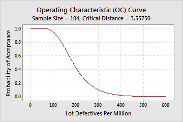
OC curve
The operating characteristic (OC) curve shows the ability of an acceptance sampling plan to distinguish between good and bad quality lots. The OC curve plots the probability of accepting lots that have different incoming quality levels for each sampling plan.
Interpretation
In this example, if the actual defectives per million is 100, you have a 0.950 probability of accepting this lot based on the sample and a 0.050 probability of rejecting it. If the actual defectives per million is 300, you have a 0.100 probability of accepting this lot and a 0.900 probability of rejecting it.
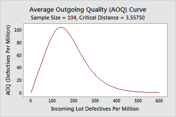
AOQ curve
The average outgoing quality (AOQ) curve shows the relationship between the quality of the incoming material and the quality of the outgoing material, assuming that rejected lots will be 100% inspected and defective items will be replaced or reworked and inspected again (rectifying inspection).
Interpretation
In this example, when the average incoming quality level is 100 defectives per million, the average outgoing quality is 91.1 defectives per million. When the average incoming quality level is 300 defectives per million, the average outgoing quality is 28.6 defectives per million. The incoming quality is worse than the outgoing quality because rejected lots will be 100% inspected and will have all nonconforming units replaced or reworked.
The worst average outgoing defective level (AOQL) of 104.6 defectives per million occurs when the incoming quality level is 140.0 defectives per million.
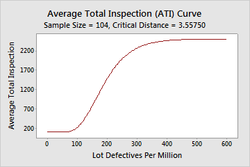
ATI curve
The average total inspection (ATI) curve shows the relationship between the quality of the incoming material and the number of items that need to be inspected, assuming that rejected lots will be 100% inspected and defective items will be replaced or reworked and inspected again (rectifying inspection).
Interpretation
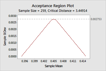
Acceptance region plot
The acceptance region plot is used for illustrating sample requirements. When the upper and lower specifications are known, and the standard deviation is unknown, the acceptance region plot lets you see the region of sample means and sample standard deviations for which you will accept a lot.
Interpretation
As the sample standard deviation increases and approaches the maximum, the mean needs to be on target for you to accept a shipment. If the process variation is tight and the standard deviation is small, the mean can vary between the specification limits.