Note
This command is available with the Predictive Analytics Module. Click here for more information about how to activate the module.
A team of researchers collects data from the sale of individual residential properties in Ames, Iowa. The researchers want to identify the variables that affect the sale price. Variables include the lot size and various features of the residential property. The researchers want to assess how well the best MARS® model fits the data.
- Open the sample data, AmesHousing.mtw.
- Select .
- In Response, enter 'Sale Price'.
- In Continuous predictors, enter 'Lot Frontage' – 'Year Sold'.
- In Categorical predictors, enter Type – 'Sale Condition'.
- Click OK.
Interpret the results
By default, MARS® Regression fits an additive model so all the basis functions in the regression equation use 1 predictor. The first predictor in the list is BF2. BF2 uses the predictor Living Area SF. Because the predictor is in 1 basis function, the predictor has 2 different slopes in the model. The function max(0, 3078 - Living Area SF) defines that the slope is non-zero when the living area is less than 3,078.
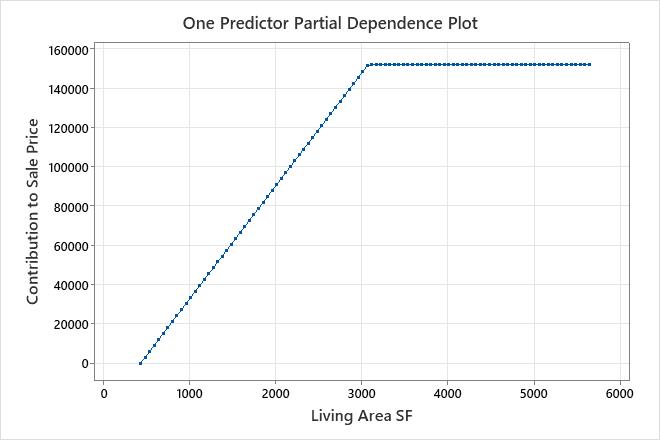
The results for an additive model include partial dependence plots for continuous predictors that are important in the model. Use the plot to see the effect of all the basis functions for a predictor across the range of the predictor. In these results, the partial dependence plot shows that for a value of Living Area SF from 438 to 3,078, the slope is about 57.6. When Living Area SF is greater than 3,078, the slope is 0.
In these results, BF2 has a negative coefficient in the regression equation. The arrangement of the basis function is max(0, c - X). In this arrangement, the value of the basis function decreases when the predictor increases. The combination of this arrangement and the negative coefficient creates a positive relationship between the predictor variable and the response variable. The effect of Living Area SF is to increase Sale Price in the region from 438 to 3,078.
The analysis also includes categorical predictors. For example, BF3 is for the predictor Quality. The basis function is for when the value of Quality is 8, 9, or 10. The coefficient for BF3 in the equation is 115,438. This basis function indicates that when the value of quality changes from a value of 1 to 7 to a value of 8, 9, or 10, the sale price increases by $115,438 in the model. Quality is also in BF11 and BF25. To understand the effect of the predictor on the response variable, consider all the basis functions.
Two of the predictors that are important in the model have missing values in the training data: Basement SF 1 and Total Basement SF. The list of basis functions includes basis functions that identify when these predictors are missing: BF7 and BF17. When either predictor has a missing value, the basis function for the indicator variable nullifies the other basis functions for that predictor through multiplication by 0.
Regression Equation
BF3 = when Quality is 8, 9, 10
BF6 = max(0, 2002 - Year Built)
BF7 = when Basement SF 1 is not missing
BF10 = max(0, 1696 - Basement SF 1) * BF7
BF11 = when Quality is 1, 8
BF13 = when Type is 90, 150, 160, 180, 190
BF15 = when Neighborhood is Blueste, ClearCr, Crawfor, GrnHill, Landmrk, NoRidge, NridgHt,
Somerst, StoneBr, Timber, Veenker
BF17 = when Total Basement SF is not missing
BF19 = max(0, Total Basement SF - 1392) * BF17
BF21 = max(0, 1st Floor SF - 2402)
BF23 = when Condition is 1, 2, 3, 4, 5, 6
BF25 = when Quality is 1, 7, 10
BF27 = max(0, 1st Floor SF - 2207)
BF30 = max(0, 15138 - Lot Area)
Sale Price = 325577 - 57.6167 * BF2 + 115438 * BF3 - 605.079 * BF6 - 25.3989 * BF10 -
66735.2 * BF11 - 23688.9 * BF13 + 22374.5 * BF15 + 50.3801 * BF19 - 576.789 * BF21 - 18099.2
* BF23 + 22414.2 * BF25 + 361.254 * BF27 - 1.82 * BF30
Note
In these results, the list of basis functions has 15 basis functions but the optimal number of basis functions is 13. The regression equation contains 13 basis functions. The list of basis functions contains BF7 and BF17, which are the basis functions that identify the missing values. These basis functions are not important on their own because they did not reduce the MSE as much as other basis functions in the search. These 2 basis functions are in the list to show the full calculation of BF10 and BF 19, which are important.
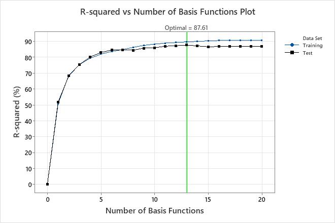
The R-squared vs Number of Basis Functions plot shows the result of the backwards elimination to find the optimal number of basis functions. To use a model with a different number of basis functions, select Select an Alternative Model. For example, if a model with much fewer basis functions is almost as accurate as the optimal model, consider whether to use the simpler model. In these results, the R-squared values for the training and test data sets are the same for the model with 7 basis functions. This smaller model is of interest if overfitting is a concern.
Model Summary
| Total predictors | 77 |
|---|---|
| Important predictors | 10 |
| Maximum number of basis functions | 30 |
| Optimal number of basis functions | 13 |
| Statistics | Training | Test |
|---|---|---|
| R-squared | 89.61% | 87.61% |
| Root mean squared error (RMSE) | 25836.5197 | 27855.6550 |
| Mean squared error (MSE) | 667525749.7185 | 775937512.8264 |
| Mean absolute deviation (MAD) | 17506.0038 | 17783.5549 |
The model summary table includes measures of how well the model performs. You can use these values to compare models. For these results, the test R-squared is about 88%.
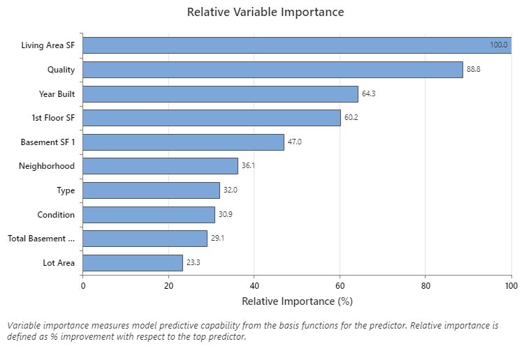
The relative variable importance chart plots the predictors in order of their effect on the model. The most important predictor variable is Living Area SF. If the contribution of the top predictor variable, Living Area SF, is 100%, then the next important variable, Quality has a contribution of 88.8%. This contribution means that Quality is 88.8% as important as Living Area SF in this model.
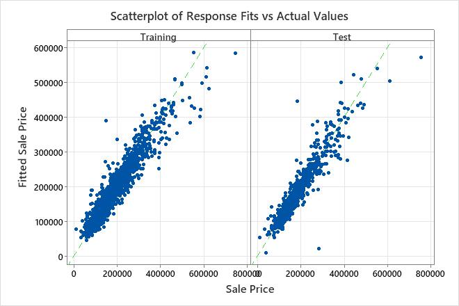
The scatterplot of fitted sale prices versus actual sale prices shows the relationship between the fitted and actual values for both the training data and the test data. You can hover over the points on the graph to see the plotted values more easily. In this example, most of the points fall approximately near the reference line of y=x.
The model fits a few distinct points poorly, such as the one in the test data set that has a fitted sale price of less than $100,000 but an actual sale price closer to $250,000. Consider whether to investigate this case to improve the fit of the model.