In This Topic
Moving average
To calculate a moving average, Minitab averages consecutive groups of observations in a series. For example, suppose a series begins with the numbers 4, 5, 8, 9, 10 and you use the moving average length of 3. The first two values of the moving average are missing. The third value of the moving average is the average of 4, 5, 8; the fourth value is the average of 5, 8, 9; the fifth value is the average of 8, 9, 10.
Centered moving average
By default, moving average values are placed at the period in which they are calculated. For example, for a moving average length of 3, the first numeric moving average value is placed at period 3, the next at period 4, and so on.
When you center the moving averages, they are placed at the center of the range rather than the end of it. This is done to position the moving average values at their central positions in time.
If the moving average length is odd
Suppose the moving average length is 3. In that case, Minitab places the first numeric moving average value at period 2, the next at period 3, and so on. In this case, the moving average value for the first and last periods is missing ( *).
If the moving average length is even
Suppose the moving average length is 4. Because you cannot place a moving average value at period 2.5, Minitab calculates the average of the first four values and names it MA1. Then Minitab calculates the average of the next four values and names it MA2. The average of those two values is the number Minitab and places at period 3. In this case, the moving average values for the first two and last two periods are missing (*).
Forecasts
The fitted value at time t is the uncentered moving average at time t – 1. The forecasts are the fitted values at the forecast origin. If you forecast 10 time units ahead, the forecasted value for each time will be the fitted value at the origin. Data up to the origin are used for calculating the moving averages.
You can use the linear moving average method by performing consecutive moving averages. This is often done when there is a trend in the data. First, compute and store the moving average of the original series. Then compute and store the moving average of the previously stored column to obtain a second moving average.
In naive forecasting, the forecast for time t is the data value at time t – 1. Using moving average procedure with a moving average of length one gives naive forecasting.
Prediction limits
Formula
Upper limit = Forecast + 1.96 × 
Lower limit = Forecast – 1.96 × 
Notation
| Term | Description |
|---|---|
| MSD | mean squared deviation |
MAPE
Mean absolute percentage error (MAPE) measures the accuracy of fitted time series values. MAPE expresses accuracy as a percentage.
Formula
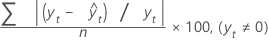
Notation
| Term | Description |
|---|---|
| yt | actual value at time t |
 | fitted value |
| n | number of observations |
MAD
Mean absolute deviation (MAD) measures the accuracy of fitted time series values. MAD expresses accuracy in the same units as the data, which helps conceptualize the amount of error.
Formula
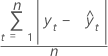
Notation
| Term | Description |
|---|---|
| yt | actual value at time t |
 | fitted value |
| n | number of observations |
MSD
Mean squared deviation (MSD) is always computed using the same denominator, n, regardless of the model. MSD is a more sensitive measure of an unusually large forecast error than MAD.
Formula
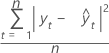
Notation
| Term | Description |
|---|---|
| yt | actual value at time t |
 | fitted value |
| n | number of observations |