Analysis of variance
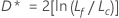
The deviance table is constructed based on the following general result which assumes that ϕ is known. If DI is the deviance associated with an initial model and DS is the deviance associated with a subset of terms in the initial model, then under some regularity conditions, the following relationship exists:

The difference between the deviances is asymptotically distributed as a chi-square distribution with d degrees of freedom. These statistics are calculated for adjusted (type III) analysis and sequential (type I) analysis. The adjusted deviance and the chi-square statistic in the deviance table are equal. The adjusted mean deviance is the adjusted deviance divided by the degrees of freedom.
For the sequential analysis, the output depends on the order that the predictors enter the model. The sequential deviance is the unique portion of the deviance that a predictor explains, given any predictors already in the model. If you have a model with three predictors, X1, X2, and X3, the sequential deviance for X3 shows how much of the remaining deviance that X3 explains given that X1 and X2 are already in the model. To obtain a different sequential deviance, repeat the regression procedure entering the predictors in a different order.
If ϕ is unknown, as for responses that follow a normal distribution, then under some regularity conditions the relationship changes to the following:
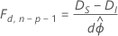
Here, the difference between the deviances is asymptotically distributed as an F distribution with d degrees of freedom for the numerator and n − p degrees of freedom for the denominator. To estimate the dispersion parameter, use the initial model.
Notation
| Term | Description |
|---|---|
| yi | the number of events for the ith row |
 | the estimated mean response of the ith row |
| mi | the number of trials for the ith row |
| Lf | the log-likelihood of the full model |
| Lc | the log likelihood of the model with a subset of terms from the full model |
| d | the degrees of freedom are the difference between the numbers of parameters in the models to compare |
| ϕ | the dispersion parameter, known to be 1 for the binomial model |
| n | the number of rows in the data |
| p | the regression degrees of freedom for the initial model |
Degrees of freedom (DF)
Different sums of squares have different degrees of freedom.
DF for a numeric factor = 1
DF for a categorical factor = b − 1
DF for a quadratic term = 1
DF for blocks = c − 1
DF for error = n − p
DF total = n − 1


Note
Categorical factors in screening designs in Minitab have 2 levels. Thus, the degrees of freedom for a categorical factor are 2 – 1 = 1. By extension, interactions between factors also have 1 degree of freedom.
Notation
| Term | Description |
|---|---|
| b | The number of levels in the factor |
| c | The number of blocks |
| n | The total number of rows in the design |
| ni | The number of observations for ith factor level combination |
| m | The number of factor level combinations |
| p | The number of coefficients |
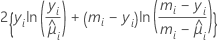
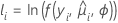
Log-likelihood
The general form of the individual contributions follows:

Notation
| Term | Description |
|---|---|
| yi | the number of events for the ith row |
| mi | the number of trials for the ith row |
 | the estimated mean response of the ith row |
p-value (P)
Used in hypothesis tests to help you decide whether to reject or fail to reject a null hypothesis. The p-value is the probability of obtaining a test statistic that is at least as extreme as the actual calculated value, if the null hypothesis is true. A commonly used cut-off value for the p-value is 0.05. For example, if the calculated p-value of a test statistic is less than 0.05, you reject the null hypothesis.