In This Topic
Step 1. Determine the number of components in the model
The objective with PLS is to select a model with the appropriate number of components that has good predictive ability. When you fit a PLS model, you can perform cross-validation to help you determine the optimal number of components in the model. With cross-validation, Minitab selects the model with the highest predicted R2 value. If you do not use cross-validation, you can specify the number of components to include in the model or use the default number of components. The default number of components is 10 or the number of predictors in your data, whichever is less. Examine the Method table to determine how many components Minitab included in the model. You can also examine the Model selection plot.
When using PLS, select a model with the smallest number of components that explain a sufficient amount of variability in the predictors and the responses. To determine the number of components that is best for your data, examine the Model selection table, including the X-variance, R2, and predicted R2 values. Predicted R2 indicates the predictive ability of the model and is only displayed if you perform cross-validation.
In some cases, you may decide to use a different model than the one initially selected by Minitab. If you used cross-validation, compare the R2 and predicted R2. Consider an example where removing two components from the model that Minitab only slightly decreases predicted R2. Because the predicted R2 only decreased slightly, the model is not overfit and you may decide it better suits your data.
A predicted R2 that is substantially less than R2 may indicate that the model is over-fit. An over-fit model occurs when you add terms or components for effects that are not important in the population, although they may appear important in the sample data. The model becomes tailored to the sample data and, therefore, may not be useful for making predictions about the population.
If you do not use cross-validation, you can examine the x-variance values in the Model selection table to determine how much variance in the response is explained by each model.
Method
| Cross-validation | Leave-one-out |
|---|---|
| Components to evaluate | Set |
| Number of components evaluated | 10 |
| Number of components selected | 4 |
Method
| Cross-validation | None |
|---|---|
| Components to calculate | Set |
| Number of components calculated | 10 |
Key Result: Number of components
In these results, in the first Method table cross-validation was used and selected the model with 4 components. In the second Method table, cross-validation was not used. Minitab uses the model with 10 components, which is the default.
Model Selection and Validation for Aroma
| Components | X Variance | Error | R-Sq | PRESS | R-Sq (pred) |
|---|---|---|---|---|---|
| 1 | 0.158849 | 14.9389 | 0.637435 | 23.3439 | 0.433444 |
| 2 | 0.442267 | 12.2966 | 0.701564 | 21.0936 | 0.488060 |
| 3 | 0.522977 | 7.9761 | 0.806420 | 19.6136 | 0.523978 |
| 4 | 0.594546 | 6.6519 | 0.838559 | 18.1683 | 0.559056 |
| 5 | 5.8530 | 0.857948 | 19.2675 | 0.532379 | |
| 6 | 5.0123 | 0.878352 | 22.3739 | 0.456988 | |
| 7 | 4.3109 | 0.895374 | 24.0041 | 0.417421 | |
| 8 | 4.0866 | 0.900818 | 24.7736 | 0.398747 | |
| 9 | 3.5886 | 0.912904 | 24.9090 | 0.395460 | |
| 10 | 3.2750 | 0.920516 | 24.8293 | 0.397395 |
Key Result: X Variance, R-sq, R-sq (pred)
In these results, Minitab selected the 4-component model which has a predicted R2 value of approximately 56%. Based on the x-variance, the 4-component model explains almost 60% of the variance in the predictors. As the number of components increases, the R2 value increases, but the predicted R2 decreases, which indicates that models with more components are likely to be over-fit.
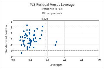
Step 2. Determine whether the data contain outliers or leverage points
To determine whether your model fits the data well, you need to examine plots to look for outliers, leverage points, and other patterns. If your data contain many outliers or leverage points, the model may not make valid predictions.
- Outliers: Observations with large standardized residuals fall outside the horizontal reference lines on the plot.
- Leverage points: Observations with leverage values have x-scores far from zero and are to the right of the vertical reference line.
For more information on the residual vs leverage plot, go to Graphs for Partial Least Squares Regression.
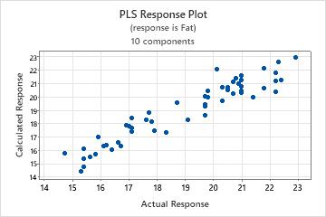
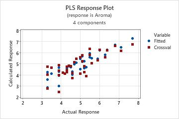
- A nonlinear pattern in the points, which indicates the model may not fit or predict data well.
- If you perform cross-validation, large differences in the fitted and the cross-validated values, which indicate a leverage point.
Step 3. Validate the PLS model with a test data set
Often, PLS regression is performed in two steps. The first step, sometimes called training, involves calculating a PLS regression model for a sample data set (also called a training data set). The second step involves validating this model with a different set of data, often called a test data set. To validate the model with the test data set, enter the columns of the test data in the Prediction sub-dialog box. Minitab calculates new response values for each observation in the test data set and compares the predicted response to the actual response. Based on the comparison, Minitab calculates the test R2, which indicates the model's ability to predict new responses. Higher test R 2 values indicate the model has greater predictive ability.
If you use cross-validation, compare the test R2 to the predicted R2. Ideally, these values should be similar. A test R2 that is significantly smaller than the predicted R2 indicates that cross-validation is overly optimistic about the model's predictive ability or that the two data samples are from different populations.
If the test data set does not include response values, then Minitab does not calculate a test R2.
Predicted Response for New Observations Using Model for Fat
| Row | Fit | SE Fit | 95% CI | 95% PI |
|---|---|---|---|---|
| 1 | 18.7372 | 0.378459 | (17.9740, 19.5004) | (16.8612, 20.6132) |
| 2 | 15.3782 | 0.362762 | (14.6466, 16.1098) | (13.5149, 17.2415) |
| 3 | 20.7838 | 0.491134 | (19.7933, 21.7743) | (18.8044, 22.7632) |
| 4 | 14.3684 | 0.544761 | (13.2698, 15.4670) | (12.3328, 16.4040) |
| 5 | 16.6016 | 0.348485 | (15.8988, 17.3044) | (14.7494, 18.4538) |
| 6 | 20.7471 | 0.472648 | (19.7939, 21.7003) | (18.7861, 22.7080) |
Key Result: Test R 2
In these results, the test R2 is approximately 76%. The predicted R2 for the original data set is approximately 78%. Because these values are similar, you can conclude that the model has adequate predictive ability.