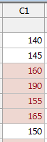
Overview for Conditional Formatting

Use Conditional Formatting to apply formatting, such as colored shading, to cells in a column based on their values. For example, in the following worksheet, cells in C1 that contain values greater than 150 have red shading and text.

You can apply more than one rule to a column. For example, for a column of test scores, you can apply one rule that formats cells that contain passing scores as green. You can then apply an additional rule to the same column that formats cells that contain failing scores as red. Conditional formatting rules are reapplied when the worksheet view refreshes.

Tip

You can subset a worksheet by rows that contain cell formatting. Click in the worksheet, then right-click and choose Subset Worksheet > Include Rows with Formatted Cells, or Subset Worksheet > Exclude Rows with Formatted Cells.

Where to find these commands

To apply conditional formatting to a column, do one of the following:

Choose Data > Conditional Formatting, then choose a rule.
Click in the column, choose Conditional Formatting, then choose a rule.
Click in the column, right-click, choose Conditional Formatting, then choose a rule.

To manage conditional formatting rules for a column, do one of the following:

Choose Data > Conditional Formatting > Manage Rules.
Click in the column, then choose Conditional Formatting > Manage Rules.
Click in the column, right-click, then choose Conditional Formatting > Manage Rules.

When to use an alternate command

If you want to apply formatting to adjacent cells manually, regardless of the values, select the cells, then right-click and choose Cell Properties > highlight option.