In This Topic
Step 1: Determine the number of factors
- % Var
- Use the percentage of variance (% Var) to determine the amount of variance that the factors explain. Retain the factors that explain an acceptable level of variance. The acceptable level depends on your application. For descriptive purposes, you may need only 80% of the variance explained. However, if you want to perform other analyses on the data, you may want to have at least 90% of the variance explained by the factors.
- Variance (Eigenvalues)
- If you use principal components to extract factors, the variance equals the eigenvalue. You can use the size of the eigenvalue to determine the number of factors. Retain the factors with the largest eigenvalues. For example, using the Kaiser criterion, you use only the factors with eigenvalues that are greater than 1.
- Scree plot
- The scree plot orders the eigenvalues from largest to smallest. The ideal pattern is a steep curve, followed by a bend, and then a straight line. Use the components in the steep curve before the first point that starts the line trend.
Unrotated Factor Loadings and Communalities
| Variable | Factor1 | Factor2 | Factor3 | Factor4 | Factor5 | Factor6 | Factor7 | Factor8 |
|---|---|---|---|---|---|---|---|---|
| Academic record | 0.726 | 0.336 | -0.326 | 0.104 | -0.354 | -0.099 | 0.233 | 0.147 |
| Appearance | 0.719 | -0.271 | -0.163 | -0.400 | -0.148 | -0.362 | -0.195 | -0.151 |
| Communication | 0.712 | -0.446 | 0.255 | 0.229 | -0.319 | 0.119 | 0.032 | 0.088 |
| Company Fit | 0.802 | -0.060 | 0.048 | 0.428 | 0.306 | -0.137 | -0.067 | 0.105 |
| Experience | 0.644 | 0.605 | -0.182 | -0.037 | -0.092 | 0.317 | -0.209 | -0.102 |
| Job Fit | 0.813 | 0.078 | -0.029 | 0.365 | 0.368 | -0.067 | -0.025 | -0.032 |
| Letter | 0.625 | 0.327 | 0.654 | -0.134 | 0.031 | 0.025 | 0.017 | -0.113 |
| Likeability | 0.739 | -0.295 | -0.117 | -0.346 | 0.249 | 0.140 | 0.353 | -0.142 |
| Organization | 0.706 | -0.540 | 0.140 | 0.247 | -0.217 | 0.136 | -0.080 | -0.105 |
| Potential | 0.814 | 0.290 | -0.326 | 0.167 | -0.068 | -0.073 | 0.048 | -0.112 |
| Resume | 0.709 | 0.298 | 0.465 | -0.343 | -0.022 | -0.107 | 0.024 | 0.170 |
| Self-Confidence | 0.719 | -0.262 | -0.294 | -0.409 | 0.175 | 0.179 | -0.159 | 0.230 |
| Variance | 6.3876 | 1.4885 | 1.1045 | 1.0516 | 0.6325 | 0.3670 | 0.3016 | 0.2129 |
| % Var | 0.532 | 0.124 | 0.092 | 0.088 | 0.053 | 0.031 | 0.025 | 0.018 |
| Variable | Factor9 | Factor10 | Factor11 | Factor12 | Communality |
|---|---|---|---|---|---|
| Academic record | 0.097 | -0.142 | -0.026 | -0.031 | 1.000 |
| Appearance | 0.082 | 0.016 | 0.020 | -0.038 | 1.000 |
| Communication | 0.023 | 0.204 | 0.012 | -0.100 | 1.000 |
| Company Fit | -0.019 | -0.067 | 0.188 | -0.021 | 1.000 |
| Experience | 0.121 | 0.039 | 0.077 | 0.009 | 1.000 |
| Job Fit | 0.146 | 0.066 | -0.176 | 0.008 | 1.000 |
| Letter | -0.079 | -0.130 | -0.043 | -0.127 | 1.000 |
| Likeability | 0.051 | 0.022 | 0.064 | 0.012 | 1.000 |
| Organization | -0.020 | -0.162 | -0.032 | 0.136 | 1.000 |
| Potential | -0.290 | 0.100 | -0.023 | 0.028 | 1.000 |
| Resume | 0.008 | 0.090 | 0.010 | 0.156 | 1.000 |
| Self-Confidence | -0.098 | -0.061 | -0.065 | -0.047 | 1.000 |
| Variance | 0.1557 | 0.1379 | 0.0851 | 0.0750 | 12.0000 |
| % Var | 0.013 | 0.011 | 0.007 | 0.006 | 1.000 |
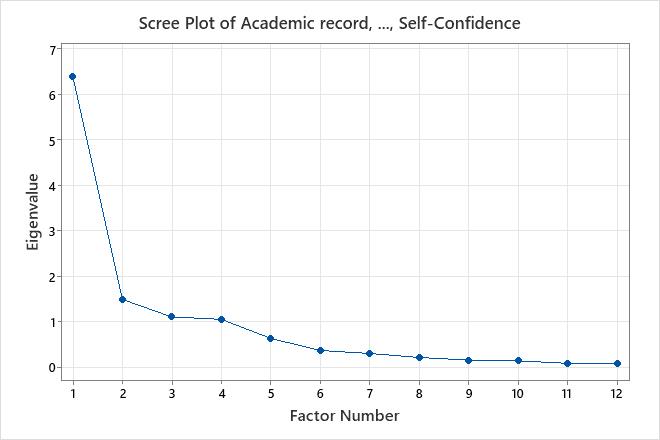
Key Results: %Var, Variance (Eigenvalue), Scree Plot
These results show the unrotated factor loadings for all the factors using the principal components method of extraction. The first four factors have variances (eigenvalues) that are greater than 1. The eigenvalues change less markedly when more than 6 factors are used. Therefore, 4–6 factors appear to explain most of the variability in the data. The percentage of variability explained by factor 1 is 0.532 or 53.2%. The percentage of variability explained by Factor 4 is 0.088 or 8.8%. The scree plot shows that the first four factors account for most of the total variability in data. The remaining factors account for a very small proportion of the variability and are likely unimportant.
Step 2: Interpret the factors
After you determine the number of factors (step 1), you can repeat the analysis using the maximum likelihood method. Then examine the loading pattern to determine the factor that has the most influence on each variable. Loadings close to -1 or 1 indicate that the factor strongly influences the variable. Loadings close to 0 indicate that the factor has a weak influence on the variable. Some variables may have high loadings on multiple factors.
Unrotated factor loadings are often difficult to interpret. Factor rotation simplifies the loading structure, allowing you to more easily interpret the factor loadings. However, one method of rotation may not work best in all cases. You may want to try different rotations and use the one that produces the most interpretable results. You can also sort the rotated loadings to more clearly assess the loadings within a factor.
Rotated Factor Loadings and Communalities
| Variable | Factor1 | Factor2 | Factor3 | Factor4 | Communality |
|---|---|---|---|---|---|
| Academic record | 0.481 | 0.510 | 0.086 | 0.188 | 0.534 |
| Appearance | 0.140 | 0.730 | 0.319 | 0.175 | 0.685 |
| Communication | 0.203 | 0.280 | 0.802 | 0.181 | 0.795 |
| Company Fit | 0.778 | 0.165 | 0.445 | 0.189 | 0.866 |
| Experience | 0.472 | 0.395 | -0.112 | 0.401 | 0.553 |
| Job Fit | 0.844 | 0.209 | 0.305 | 0.215 | 0.895 |
| Letter | 0.219 | 0.052 | 0.217 | 0.947 | 0.994 |
| Likeability | 0.261 | 0.615 | 0.321 | 0.208 | 0.593 |
| Organization | 0.217 | 0.285 | 0.889 | 0.086 | 0.926 |
| Potential | 0.645 | 0.492 | 0.121 | 0.202 | 0.714 |
| Resume | 0.214 | 0.365 | 0.113 | 0.789 | 0.814 |
| Self-Confidence | 0.239 | 0.743 | 0.249 | 0.092 | 0.679 |
| Variance | 2.5153 | 2.4880 | 2.0863 | 1.9594 | 9.0491 |
| % Var | 0.210 | 0.207 | 0.174 | 0.163 | 0.754 |
Key Results: Loadings, communality, loading plot
- Company Fit (0.778), Job Fit (0.844), and Potential (0.645) have large positive loadings on factor 1, so this factor describes employee fit and potential for growth in the company.
- Appearance (0.730), Likeability (0.615), and Self-confidence (0.743) have large positive loadings on factor 2, so this factor describes personal qualities.
- Communication (0.802) and Organization (0.889) have large positive loadings on factor 3, so this factor describes work skills.
- Letter (0.947) and Resume (0.789) have large positive loadings on factor 4, so this factor describes writing skills.
Together, all four factors explain 0.754 or 75.4% of the variation in the data.
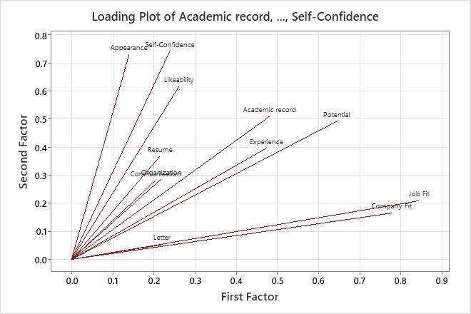
The loading plot visually shows the loading results for the first two factors.
Step 3: Check your data for problems
If the first two factors account for most of the variance in the data, you can use the score plot to assess the data structure and detect clusters, outliers, and trends. Groupings of data on the plot may indicate two or more separate distributions in the data. If the data follow a normal distribution and no outliers are present, the points are randomly distributed about the value of 0.
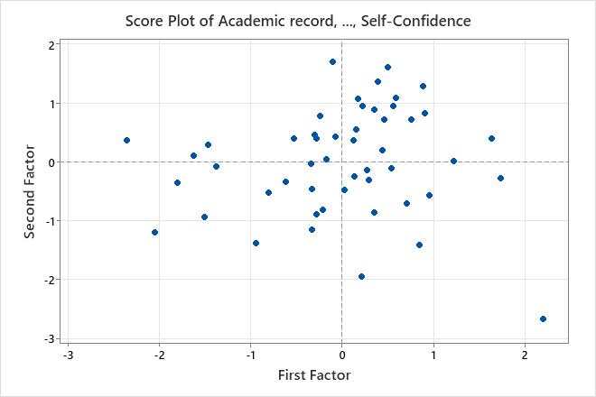
Key Result: Score Plot
In this score plot, the data appear normal and no extreme outliers are apparent. However, you may want to investigate the data value shown in the lower right of the plot, which lies farther away from the other data values.
Tip
To see the calculated score for each observation, hold your pointer over a data point on the graph. To create score plots for other factors, store the scores and use .