Interpret the key results for Response Optimizer

Complete the following steps to interpret Response Optimizer. Key output includes the optimization plot, fitted values, and the confidence intervals.

In This Topic

Step 1: Identify the optimal setting of each predictor
Step 2: Identify the point estimate and the likely range of each response

Step 1: Identify the optimal setting of each predictor

Use the optimization plot to determine the optimal settings for the predictors given the parameters that you specified. Double-click the optimization plot to make it interactive and investigate how the variables affect the predicted responses. You can modify the variable settings directly on the plot by moving the vertical red bars.

The optimization plot displays the fitted values for the predictor settings. However, you should examine the prediction intervals in the output to determine whether the range of likely values for a single future value falls within acceptable boundaries for the process.

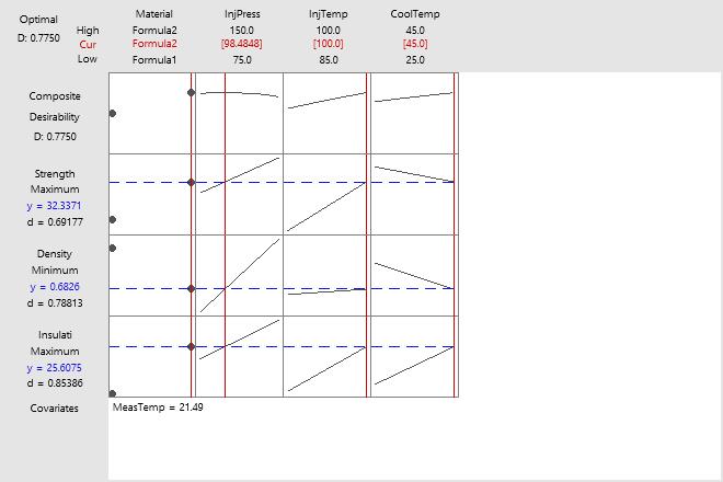
Key Result: Optimization plot

For the insulation data, the composite desirability is 0.7750. The first column of the graph shows the response values at each level of Material, which is a categorical variable. The current variable settings are Material = Formula2, InjPress = 98.4848, InjTemp = 100.0, and CoolTemp = 45.0. The goal was to Maximize Insulation. Its predicted value is 25.6075, and its individual desirability is 0.85386. The covariate, MeasTemp, is included in the model as an uncontrollable noise variable and it is held at 21.49. Further observations are as follows:

Material: The two points for each cell in this column represent the two levels of the categorical variable: Formula1 and Formula2. Formula2 appears to be the best material. Changing to Formula1 would decrease the insulative value and increase the density, which are both undesirable. However, because material type interacts with other factors, this trend might not hold at other settings. Consider whether you can find a local solution for Formula1. Or, change the settings for Formula1 directly on the graph by moving the vertical bars.

InjPress: Increasing the injection pressure increases all three responses. Therefore, the optimal setting is in the middle of the range (98.4848), which is a compromise between conflicting goals. The goal is to maximize insulative value, minimize density, and maximize strength.

InjTemp: Increasing injection temperature also increases all the responses. But the effect on density is minimal compared to the effect on insulative value. Therefore, you increase the composite desirability by maximizing the injection temperature. The optimal settings of injection temperature are at the maximum levels in the experiment. This result suggests that you should consider experimenting with higher temperatures.

CoolTemp: Increasing cooling temperature increases insulative value, but decreases both density and strength. The optimal settings of both injection temperature and cooling temperature are at the maximum levels in the experiment. This result suggests that you should consider experimenting with higher temperatures. The graphs show that higher cooling temperatures may be especially worth considering. If the graphs could be extrapolated, higher cooling temperatures would improve insulative value and density. However, strength would decrease.

Step 2: Identify the point estimate and the likely range of each response

Use the fit values to identify the point estimate of each response variable for the settings in the optimization plot.

The prediction interval (PI) is a range that is likely to contain a single future response value for a specified combination of variable settings. If you collect another data point at the same settings, the new data point is likely to be within the prediction interval. Narrower prediction intervals indicate a more precise prediction

The prediction intervals help you assess the practical significance of your results. If a prediction interval extends outside of acceptable boundaries, the predictions might not be precise enough for your requirements. In this case, consider the following options:

Search for settings that give adequate precision on the optimization plot.
Conduct additional research and consider increasing the sample size to obtain more precise predictions.

To search for better settings on the optimization plot, complete the following steps:

Double-click the optimization plot to make it interactive.
Adjust the predictor settings directly on the Optimization plot by moving the red vertical bars.
Click the Predict button on the toolbar to generate new prediction intervals to determine whether the new solution is acceptable.

Multiple Response Prediction

Variable	Setting
Material	Formula2
InjPress	98.4848
InjTemp	100
CoolTemp	45
MeasTemp	21.4875

Response	Fit	SE Fit	95% CI	95% PI
Strength	32.34	1.04	(29.45, 35.22)	(27.25, 37.43)
Density	0.6826	0.0597	(0.5167, 0.8484)	(0.3899, 0.9753)
Insulation	25.608	0.268	(24.863, 26.352)	(24.294, 26.921)

Key Results: Fit, PI

In these results, the input variable settings on the optimization plot are associated with the following predicted means and prediction intervals:

The mean strength is 32.34 and the range of likely values for a single future value is 27.25 to 37.43.
The mean density is 0.6826 and the range of likely values for a single future value is 0.3899 to 0.9753.
The mean insulation is 25.608 and the range of likely values for a single future value is 24.294 to 26.921.